(Written for release of v6.0, June 2020)

Expand

title	Click here for page contents...

Table of Contents

Child pages (Children Display)

...

Note

title	Prerequisites

It is recommended that you familiarise yourself with R first by sitting our Introduction to R tutorial.

It also requires that you have the DataSHIELD training environment installed on your machine, see our Installation Instructions for Linux, Windows, or Mac.

Tip

title	Help

DataSHIELD support is freely available in the DataSHIELD forum by the DataSHIELD community. Please use this as the first port of call for any problems you may be having, it is monitored closely for new threads.

DataSHIELD bespoke user support and also user training classes are offered on a fee-paying basis. Please enquire at datashield@newcastle.ac.uk for current prices.

Introduction

This tutorial introduces users to DataSHIELD commands and syntax. Throughout this document we refer to R, but all commands are run in the same way in Rstudio. This tutorial contains a limited number of examples; further examples are available in each DataSHIELD function manual page that can be accessed via the help function.

...

Tip

title	How assign and aggregate functions work

DataSHIELD commands call functions that range from carrying out pre-requisite tasks such as login to the datasources, to generating basic descriptive statistics, plots and tabulations. More advance functions allow for users to fit generalized linear models and generalized estimating equations models. R can list all functions available in DataSHIELD.

This section explains the functions we will call during this tutorial. Although this knowledge is not required to run DataSHIELD analyses it helps to understand the output of the commands. It can explain why some commands call functions that return nothing to the user, but rather store the output on the server of the data provider for use in a second function.

In DataSHIELD the person running an analysis (the client) uses client-side functions to issue commands (instructions). These commands initiate the execution (running) of server-side functions that run the analysis server-side (behind the firewall of the data provider). There are two types of server-side function: assign functions and aggregate functions.

Assign functions do not return an output to the client, with the exception of error or status messages. Assign functions create new objects and store them server-side either because the objects are potentially disclosive, or because they consist of the individual-level data which, in DataSHIELD, is never seen by the analyst. These new objects can include:

new transformed variables (e.g. mean centred or log transformed variables)
a new variable of a modified class (e.g. a variable of class numeric may be converted into a factor which R can then model as having discrete categorical levels)
a subset object (e.g. a dataframe including gender as a variable may be split into males and females).

Assign functions return no output to the client except to indicate an error or useful messages about the object store on server-side.

Aggregate functions analyse the data server-side and return an output in the form of aggregate data (summary statistics that are not disclosive) to the client. The help page for each function tells us what is returned and when not to expect an output on client-side.

...

Please follow instructions to Start the Opal VMs.

Recall from the installation instructions, the Opal web interface:

...

Anchor

	load_packages
	load_packages

Start R/RStudio

Load Packages

The following relevant R packages are required for analysis:

...

Code Block

	xml
	xml

#load libraries
library(DSI)
library(DSOpal)
library(dsBaseClient)

Build your login dataframe

Tip

title	DataSHIELD cloud IP addresses

The DataSHIELD cloud training environment does not use fixed IP addresses, the client and opal training server addresses change each training session. As part of the user tutorial you learn how to build a DataSHIELD login dataframe. In a real world instance of DataSHIELD this is populated with secure certificates not text based usernames and passwords.

Login Dataframe

Build login dataframe.

Code Block

language	xml
title	Build your login dataframe

builder <- DSI::newDSLoginBuilder()
builder$append(server = "study1",  url = "http://192.168.56.100:8080/",
               user = "administrator", password = "datashield_test&",
               table = "CNSIM.CNSIM1", driver = "OpalDriver")
builder$append(server = "study2", url = "http://192.168.56.101:8080/",
               user = "administrator", password = "datashield_test&",
               table = "CNSIM.CNSIM2", driver = "OpalDriver")

logindata <- builder$build()

...

Anchor

	assign_variables
	assign_variables

Assign individual variables on login

Users can specify individual variables to assign to the server-side R session. It is best practice to first create a list of the Opal variables you want to analyse.

...

Div

style	page-break-after:always;

Basic statistics and data manipulations

Descriptive statistics: variable dimensions and class

It is possible to get some descriptive or exploratory statistics about the assigned variables held in the server-side R session such as number of participants at each data provider, number of participants across all data providers and number of variables. Identifying parameters of the data will facilitate your analysis.

...

Code Block

theme	RDark

  Aggregated (exists("D")) [=============================================================] 100% / 0s
  Aggregated (classDS("D$LAB_HDL")) [====================================================] 100% / 1s
$study1
[1] "numeric"

$study2
[1] "numeric"

Descriptive statistics: quantiles and mean

As LAB_HDL is a numeric variable the distribution of the data can be explored.

...

Code Block

theme	RDark

  Aggregated (meanDS(D$LAB_HDL)) [=======================================================] 100% / 0s
$Mean.by.Study
       EstimatedMean Nmissing Nvalid Ntotal
study1      1.569416      360   1803   2163
study2      1.556648      555   2533   3088

$Nstudies
[1] 2

$ValidityMessage
       ValidityMessage 
study1 "VALID ANALYSIS"
study2 "VALID ANALYSIS"

Descriptive statistics: assigning variables

So far all the functions in this section have returned something to the screen. Some functions (assign functions) create new objects in the server-side R session that are required for analysis but do not return an anything to the client screen. For example, in analysis the log values of a variable may be required.

...

Code Block

theme	RDark

  Aggregated (meanDS(LAB_HDL.c)) [=======================================================] 100% / 0s
$Mean.by.Study
       EstimatedMean Nmissing Nvalid Ntotal
study1   0.007416316      360   1803   2163
study2  -0.005352231      555   2533   3088

$Nstudies
[1] 2

$ValidityMessage
       ValidityMessage 
study1 "VALID ANALYSIS"
study2 "VALID ANALYSIS"

Generating contingency tables

The function ds.table creates contingency tables of a categorical variables. The default is set to run on pooled data from all studies, to obtain an output of each study set the argument type='split' .

...

Code Block

language	xml
theme	RDark

$chisq.tests
$chisq.tests$chisq.test_TABLE.STUDY.1_counts

	Pearson's Chi-squared test with Yates' continuity correction

data:  input.array.source.specific
X-squared = 3.8767, df = 1, p-value = 0.04896


$chisq.tests$chisq.test_TABLE.STUDY.2_counts

	Pearson's Chi-squared test with Yates' continuity correction

data:  input.array.source.specific
X-squared = 3.5158, df = 1, p-value = 0.06079


$chisq.tests$chisq.test_TABLES.COMBINED_all.sources_counts

	Pearson's Chi-squared test with Yates' continuity correction

data:  combine.array.all.sources
X-squared = 7.9078, df = 1, p-value = 0.004922



$validity.message
[1] "Data in all studies were valid"

Generating graphs

It is currently possible to produce 4 types of graphs in DataSHIELD: histograms, contour plots, heatmap plots and scatter plots.

Anchor

	histograms
	histograms

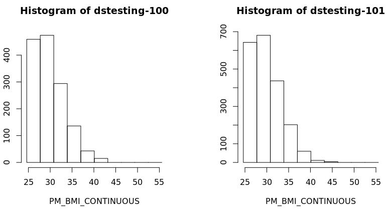
Histograms

Tip

title	Histograms

In the default method of generating a DataSHIELD histogram outliers are not shown as these are potentially disclosive. The text summary of the function printed to the client screen informs the user of the presence of classes (bins) with a count smaller than the minimal cell count set by data providers.

Note that a small random number is added to the minimum and maximum values of the range of the input variable. Therefore each user should expect slightly different printed results from those shown below:

...

Anchor

	contour_plots
	contour_plots

Contour plots

Contour plots are used to visualize a correlation pattern.

...

Anchor

	heatmap_plots
	heatmap_plots

Heat map plots

An alternative way to visualise correlation between variables is via a heat map plot.

...

Tip
The functions `ds.contourPlot` and `ds.heatmapPlot` use the range (minimum and maximum values) of the x and y vectors in the process of generating the graph. But in DataSHIELD the minimum and maximum values cannot be returned because they are potentially disclosive; hence what is actually returned for these plots is the 'obscured' minimum and maximum.

Saving Graphs / Plots in R Studio

Any plots will appear in the bottom right window in R Studio, within the plot tab
Select export > save as image

...

The plot will now be accessible from your Home folder directory structure.

Sub-setting

Tip

title	Limitations on subsetting

Sub-setting is particularly useful in statistical analyses to break down variables or tables of variables into groups for analysis. Repeated sub-setting, however, can lead to thinning of the data to individual-level records that are disclosive (e.g. the statistical mean of a single value point is the value itself). Therefore, DataSHIELD does not subset an object below the minimal subset length set by the data providers (typically this is ≤ 4 observations).

...

ds.subsetByClass
ds.dataFrameSubset
ds.subset (WARNING: this function will be deprecated in the release of 6.1, all functionallity has been added to ds.dataFrameSubset which will become the one-stop replacement).

Anchor

	sub_class
	sub_class

Sub-setting using ds.subsetByClass

The ds.subsetByClass function generates subsets for each level of a categorical variable. If the input is a data frame it produces a subset of that data frame for each class of each categorical variable held in the data frame.
Best practice is to state the categorical variable(s) to subset using the variables argument, and the name of the subset data using the subsets argument.
The example subsets GENDER from our assigned data frame D , the subset data is named GenderTables :

...

Anchor

	sub_meanbyclass
	sub_meanbyclass

Sub-setting using ds.subset

Warning

This function is soon to be deprecated. Its replacement will be ds.dataFrameSubset().

ds.dataFrameSubset() uses very different arguments to ds.subset()

Changes will be coming soon to this page. Use function help to investigate how ds.dataFrameSubset() works similarly.

...

Code Block

language	xml

ds.histogram('BMI25plus$PM_BMI_CONTINUOUS', datasources = opals)

Warning: dstesting-100: 2 invalid cells
Warning: dstesting-101: 1 invalid cells
[[1]]
$breaks
 [1] 23.93659 27.17016 30.40373 33.63731 36.87088 40.10445 43.33803 46.57160 49.80518 53.03875 56.27232
$counts
 [1] 365 511 331 150  49  15   0   0   0   0
$density
 [1] 0.079212771 0.110897880 0.071834047 0.032553194 0.010634043 0.003255319 0.000000000 0.000000000 0.000000000 0.000000000
$mids
 [1] 25.55337 28.78695 32.02052 35.25409 38.48767 41.72124 44.95482 48.18839 51.42196 54.65554
$xname
[1] "xvect"
$equidist
[1] TRUE
attr(,"class")
[1] "histogram"

[[2]]
$breaks
 [1] 23.93659 27.17016 30.40373 33.63731 36.87088 40.10445 43.33803 46.57160 49.80518 53.03875 56.27232
$counts
 [1] 506 750 476 229  62  11   4   0   0   0
$density
 [1] 0.0767450721 0.1137525773 0.0721949690 0.0347324536 0.0094035464 0.0016683711 0.0006066804 0.0000000000 0.0000000000 0.0000000000
$mids
 [1] 25.55337 28.78695 32.02052 35.25409 38.48767 41.72124 44.95482 48.18839 51.42196 54.65554
$xname
[1] "xvect"
$equidist
[1] TRUE
attr(,"class")
[1] "histogram

Modelling

Horizontal DataSHIELD allows the fitting of generalised linear models (GLM). In the GLM function the outcome can be modelled as continuous, or categorical (binomial or discrete). The error to use in the model can follow a range of distribution including gaussian, binomial, Gamma and poisson. In this section only one example will be shown, for more examples please see the manual help page for the function.

Anchor

	glm
	glm

Generalised linear models

The function ds.glm is used to analyse the outcome variable DIS_DIAB (diabetes status) and the covariates PM_BMI_CONTINUOUS (continuous BMI), LAB_HDL (HDL cholesterol) and GENDER (gender), with an interaction between the latter two. In R this model is represented as:

...

Tip

title	How ds.glm works

After every iteration in the glm, each study returns non disclosive summaries (a score vector and an information matrix) that are combined on the client R session. The model is fitted again with the updated beta coefficients, this iterative process continues until convergence or the maximum number of iterations is reached. The output of ds.glm returns the final pooled score vector and information along with some information about the convergence and the final pooled beta coefficients.

Conclusion

Tip

You have now completed our basic DataSHIELD training.

Some extended practicals will be coming soon.

Also remember you can:

get a function list for any DataSHIELD package and
view the manual help page individual functions
in the DataSHIELD test environment it is possible to print analyses to file (.csv, .txt, .pdf, .png)
take a look at our FAQ page for solutions to common problems such as Changing variable class to use in a specific DataSHIELD function.
Get support from our DataSHIELD forum.

...

Versions Compared

Old Version 64

New Version Current

Key

Introduction

Start R/RStudio

Load Packages

Build your login dataframe

Login Dataframe

Assign individual variables on login

Basic statistics and data manipulations

Descriptive statistics: variable dimensions and class

Descriptive statistics: quantiles and mean

Descriptive statistics: assigning variables

Generating contingency tables

Generating graphs

Histograms

Contour plots

Heat map plots

Saving Graphs / Plots in R Studio

Sub-setting

Sub-setting using ds.subsetByClass

Sub-setting using ds.subset

Modelling

Generalised linear models

Conclusion

Page Comparison

Versions Compared

Old Version 64

New Version Current

Key

Introduction

Start R/RStudio

Load Packages

Build your login dataframe

Login Dataframe

Assign individual variables on login

Basic statistics and data manipulations

Descriptive statistics: variable dimensions and class

Descriptive statistics: quantiles and mean

Descriptive statistics: assigning variables

Generating contingency tables

Generating graphs

Histograms

Contour plots

Heat map plots

Saving Graphs / Plots in R Studio

Sub-setting

Sub-setting using ds.subsetByClass

Sub-setting using ds.subset

Modelling

Generalised linear models

Conclusion