The answers and suggested code below are for the extended practical session that allows you to implement basic DataSHIELD functions and interpret the results.

# load libraries
library(opal)
library(dsBaseClient)
server <- c("study1", "study2", "study3")
url <- c("http://XXXXXX:8080")
table <- c("DASIM.DASIM1", "DASIM.DASIM2", "DASIM.DASIM3")
logindata <- data.frame(server, url, user="administrator", password="datashield_test&", table)
# login and assign the whole dataset
opals <- datashield.login(logins=logindata, assign=TRUE)

Subsets and Statistics

Calculate the mean and the variance of the continuous variable BMI of obese males.

# Check the levels of categorigal BMI (1=normal, 2=overweight, 3=obese)
ds.levels('D$PM_BMI_CATEGORICAL')

# Check the levels of gender (0=males, 1=females)
ds.levels('D$GENDER')

# Create a subset dataset that includes only the obese people
ds.subset(x='D', subset='BMI_3', logicalOperator='PM_BMI_CATEGORICAL==', threshold=3)

# See how many obese people are in each study
ds.dim('BMI_3')

# Create a subset dataset that includes only the obese males
ds.subset(x='BMI_3', subset='BMI_3_males', logicalOperator='GENDER==', threshold=0)

# Check how many obese males are in each study
ds.dim('BMI_3_males')

# Calculate the global mean and global variance of continuous bmi for obese males
ds.mean('BMI_3_males$PM_BMI_CONTINUOUS', type = 'combine')
ds.var('BMI_3_males$PM_BMI_CONTINUOUS', type = 'combine')

The global mean and the global variance of BMI are 33.04723 and 6.134642 respectively.

Assign and Plots

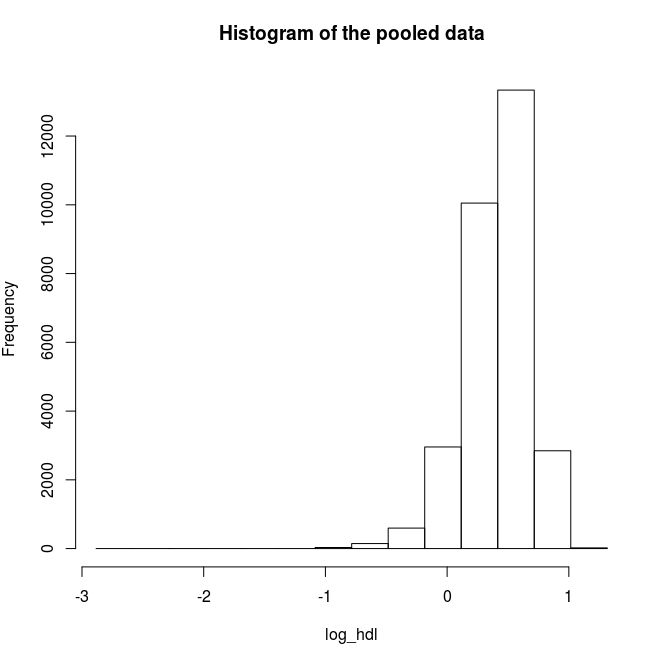
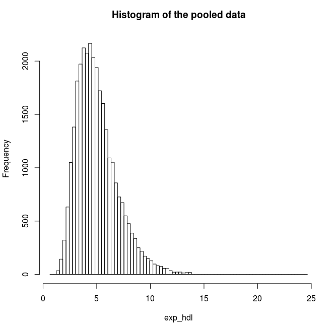
Find the quantile mean and plot a histogram of pooled data for the exponent and for the logarithm of LAB_HDL measurement.

# Assign a new variable which gives the exponents of HDL
ds.exp(x='D$LAB_HDL', newobj='exp_hdl')

# Find the quantile mean of the exponents of HDL
ds.quantileMean('exp_hdl')
 
# Plot a histogram for the exponents of HDL
ds.histogram('exp_hdl')

Quantiles of the pooled data

5% 10% 25% 50% 75% 90% 95% Mean

2.555388 2.922673 3.660593 4.727446 6.072125 7.653894 8.725955 5.066809

DataSHIELD > DataSHIELD extended practical answers - http://bit.ly/extended-DS-answers > hist1.png

# Assign a new variable which gives the logarithms of HDL
ds.log(x='D$LAB_HDL', newobj='log_hdl')

# Find the quantile mean of the logarithms of HDL
ds.quantileMean('log_hdl')
 
# Plot a histogram for the logarithms of HDL
ds.histogram('log_hdl')

Quantiles of the pooled data

5% 10% 25% 50% 75% 90%

-0.06384112 0.06994799 0.26052368 0.44043450 0.58983773 0.71059831

95% Mean

0.77301979 0.40754040

DataSHIELD > DataSHIELD extended practical answers - http://bit.ly/extended-DS-answers > hist2.png

2-dimensional contingency tables

What percentage of females (pooled data) are diabetics?
What percentage of males in each study separately have stroke (DIS_CVA)?

# Produce a two dimensional table for the variables GENDER and
# DIS_DIAB for combined data
ds.table2D(x='D$GENDER', y='D$DIS_DIAB')

1.57% of females (pooled data) are diabetics.

$counts
$counts$`pooled-D$GENDER(row)|D$DIS_DIAB(col)`
 0 1 Total
0 14830 158 14988
1 14777 235 15012
Total 29607 393 30000

$rowPercent
$rowPercent$`pooled-D$GENDER(row)|D$DIS_DIAB(col)`
 0 1 Total
0 98.95 1.05 100
1 98.43 1.57 100
Total 98.69 1.31 100

$colPercent
$colPercent$`pooled-D$GENDER(row)|D$DIS_DIAB(col)`
 0 1 Total
0 50.09 40.2 49.96
1 49.91 59.8 50.04
Total 100.00 100.0 100.00

$chi2Test
$chi2Test$`pooled-D$GENDER(row)|D$DIS_DIAB(col)`
Pearson's Chi-squared test with Yates' continuity correction
data: pooledContingencyTable
X-squared = 14.769, df = 1, p-value = 0.0001215

$validity
[1] "All tables are valid!"

# Produce a two dimensional table for the variables GENDER and 
# DIS_CVA for split data
ds.table2D(x='D$GENDER', y='D$DIS_CVA', type='split')

The percentages of males having stroke are 0.82% in study 1, 0.80% in study 2 and 0.78% in study 3.

$counts
$counts$`study1-D$GENDER(row)|D$DIS_CVA(col)`
         0  1 Total
0     4955 41  4996
1     4979 25  5004
Total 9934 66 10000

$counts$`study2-D$GENDER(row)|D$DIS_CVA(col)`
         0  1 Total
0     4956 40  4996
1     4970 34  5004
Total 9926 74 10000

$counts$`study3-D$GENDER(row)|D$DIS_CVA(col)`
         0  1 Total
0     4960 36  4996
1     4976 28  5004
Total 9936 64 10000

$rowPercent
$rowPercent$`study1-D$GENDER(row)|D$DIS_CVA(col)`
          0    1 Total
0     99.18 0.82   100
1     99.50 0.50   100
Total 99.34 0.66   100

$rowPercent$`study2-D$GENDER(row)|D$DIS_CVA(col)`
          0    1 Total
0     99.20 0.80   100
1     99.32 0.68   100
Total 99.26 0.74   100

$rowPercent$`study3-D$GENDER(row)|D$DIS_CVA(col)`
          0    1 Total
0     99.28 0.72   100
1     99.44 0.56   100
Total 99.36 0.64   100

$colPercent
$colPercent$`study1-D$GENDER(row)|D$DIS_CVA(col)`
           0      1  Total
0      49.88  62.12  49.96
1      50.12  37.88  50.04
Total 100.00 100.00 100.00

$colPercent$`study2-D$GENDER(row)|D$DIS_CVA(col)`
           0      1  Total
0      49.93  54.05  49.96
1      50.07  45.95  50.04
Total 100.00 100.00 100.00

$colPercent$`study3-D$GENDER(row)|D$DIS_CVA(col)`
           0      1  Total
0      49.92  56.25  49.96
1      50.08  43.75  50.04
Total 100.00 100.00 100.00

$chi2Test
$chi2Test$`study1-D$GENDER(row)|D$DIS_CVA(col)`
Pearson's Chi-squared test with Yates' continuity correction

data:  contingencyTable
X-squared = 3.4559, df = 1, p-value = 0.06302

$chi2Test$`study2-D$GENDER(row)|D$DIS_CVA(col)`
Pearson's Chi-squared test with Yates' continuity correction

data:  contingencyTable
X-squared = 0.34846, df = 1, p-value = 0.555

$chi2Test$`study3-D$GENDER(row)|D$DIS_CVA(col)`
Pearson's Chi-squared test with Yates' continuity correction

Generalized Linear Models

Apply a generalised linear model that predicts the level of glucose between males and females. What is the predicted average level of glucose for males? What is this value for females?
Apply a GLM to predict the level of glucose using gender and continuous bmi. How much the level of glucose is increasing with the increase of bmi by one unit? What is the predicted glucose level of a female with bmi=22?

# Apply GLM to find the linear relationship between
# LAB_GLUC_FASTING and GENDER
ds.glm("D$LAB_GLUC_FASTING ~ 1 + D$GENDER",family="gaussian")

The relationship between glucose and gender is given by the formula:
LAB_GLUC_FASTING=4.62223776-0.08929719*GENDER

For males, GENDER=0 and therefore their average level of glucose is 4.62223776

For females, GENDER=1 their average level of glucose is 4.62223776 - 0.08929719 = 4.532941

$formula
[1] "D$LAB_GLUC_FASTING ~ 1 + D$GENDER"

$family
Family: gaussian
Link function: identity

$coefficients
            Estimate    Std. Error   z-value    p-value      
(Intercept) 4.62223776  0.005806318  796.07035  0.000000e+00 
GENDER1     -0.08929719 10.008208091 -10.87917  1.448816e-27 

            low0.95CI   high0.95CI
(Intercept) 4.6108576   4.63361793
GENDER1     -0.1053848  -0.07320963

$dev
[1] 15157.85
$df
[1] 29998
$nsubs
[1] 30000
$iter
[1] 3
attr(,"class")
[1] "glmds"

# Apply GLM to find the linear relationship of LAB_GLUC_FASTING
# with GENDER and PM_BMI_CONTINUOUS
ds.glm("D$LAB_GLUC_FASTING~1+D$GENDER+D$PM_BMI_CONTINUOUS", family="gaussian")

The level of glucose related to gender and bmi is given by the formula:
LAB_GLUC_FASTING=3.64750965-0.07493214*GENDER+0.03543909*PM_BMI_CONTINUOUS

While the level of bmi is increasing by one unit, the level of glucose is increasing by 0.03543909.

For a female (GENDER=1) with PM_BMI_CONTINUOUS=22, the level of glucose should be
3.64750965 - 0.07493214 * 1 + 0.03543909 * 22 = 4.352237

$formula
[1] "D$LAB_GLUC_FASTING ~ 1 + D$GENDER + D$PM_BMI_CONTINUOUS"

$family
Family: gaussian
Link function: identity

$coefficients
                  Estimate    Std. Error    z-value     p-value     
(Intercept)       3.64750965  0.0237582722  153.525880  0.000000e+00  
GENDER1           -0.07493214 0.0079817991  -9.387876   6.122208e-21  
PM_BMI_CONTINUOUS 0.03543909  0.0008390991  42.234690 0.000000e+00  

                  low0.95CI   high0.95CI
(Intercept)       3.60094429  3.6940750
GENDER1           -0.09057618 -0.0592881
PM_BMI_CONTINUOUS 0.03379449  0.0370837

$dev
[1] 14307.08
$df
[1] 29997
$nsubs
[1] 30000
$iter
[1] 3
attr(,"class")
[1] "glmds"

# clear the Datashield R sessions and logout 
datashield.logout(opals)