Tip

title	Help

DataSHIELD support is freely available in the DataSHIELD forum by the DataSHIELD community. Please use this as the first port of call for any problems you may be having, it is monitored closely for new threads.

DataSHIELD bespoke user support and also user training classes are offered on a fee-paying basis. Please enquire at datashield@newcastle.ac.uk for current prices.

Introduction

This is the fifth in a 6-part DataSHIELD tutorial series.

The other parts in this DataSHIELD tutorial series are:

1: Introduction and logging in
2: Basic statistics and data manipulations
3: Assign functions and tables
4: Plotting graphs
5: Sub-setting
6: Modelling

Quick reminder for logging in:

Expand

Follow instructions to Start the Opal VMs.

Recall from the installation instructions, the Opal web interface is a simple check to tell if the VMs have started. Load the following urls, waiting at least 1 minute after starting the training VMs.

Start R/RStudio

Load Packages

Code Block

	xml
	xml

#load libraries
library(DSI)
library(DSOpal)
library(dsBaseClient)

Build your login dataframe

Code Block

language	xml
title	Build your login dataframe

builder <- DSI::newDSLoginBuilder()
builder$append(server = "study1",  url = "http://192.168.56.100:8080/",
               user = "administrator", password = "datashield_test&",
               table = "CNSIM.CNSIM1", driver = "OpalDriver")
builder$append(server = "study2", url = "http://192.168.56.101:8080/",
               user = "administrator", password = "datashield_test&",
               table = "CNSIM.CNSIM2", driver = "OpalDriver")

logindata <- builder$build()

connections <- DSI::datashield.login(logins = logindata, assign = TRUE, symbol = "D")

Command to logout:

Code Block

language	bash

DSI::datashield.logout(connections)

Sub-setting

Tip

title	Limitations on subsetting

Sub-setting is particularly useful in statistical analyses to break down variables or tables of variables into groups for analysis. Repeated sub-setting, however, can lead to thinning of the data to individual-level records that are disclosive (e.g. the statistical mean of a single value point is the value itself). Therefore, DataSHIELD does not subset an object below the minimal subset length set by the data providers (typically this is ≤ 4 observations).

In DataSHIELD there is one function that allows subsetting sub-setting of data, ds.dataFrameSubset .

...

Subset a column of data by its "Class"
Subset a dataframe to remove any "NA"s
Subset a numeric column of a dataframe using a Boolean inequalilty

Sub-setting by class

You may wish to generate subsets for each level of a categorical variable. To do this we must think about which levels of that categorical variable are available, then use boolean operators to isolate them:

...

Now there are two serverside objects which have split GENDER by class, to which we have assigned the names "CNSIM.subset.Males" and "CNSIM.subset.Females".

Other general examples of sub-setting

The function ds.dataFrameSubset allows general sub-setting of different data types e.g. categorical, numeric, character, data frame, matrix. It is also possible to subset rows (the individual records). No output is returned to the client screen, the generated subsets are stored in the server-side R session.

The example below uses the function ds.dataFrameSubset to subset the assigned data frame D by rows (individual records) that have no missing values (missing values are denoted with NA ) given by the argument completeCases=TRUE . The output subset is named "D_without_NA":

Sub-set by inequality

Say we wanted to have a subset where BMI values are ≥ 25, and call it subset.BMI.25.plus

...

Expand

title	Deprecated instructions on ds.subset and ds.subsetByClass, soon to be replaced with instructions using ds.dataFrameSubset

In DataSHIELD there are currently 3 functions that allow us to generate subset data:

ds.subsetByClass (WARNING: this function will be deprecated in the release of 6.1, all functionality has been added to ds.dataFrameSubset which will become the one-stop replacement)
ds.subset (WARNING: this function will be deprecated in the release of 6.1, all functionality has been added to ds.dataFrameSubset which will become the one-stop replacement).
ds.dataFrameSubset

Anchor

	sub_class
	sub_class

Sub-setting using ds.subsetByClass

The ds.subsetByClass function generates subsets for each level of a categorical variable. If the input is a data frame it produces a subset of that data frame for each class of each categorical variable held in the data frame.
Best practice is to state the categorical variable(s) to subset using the variables argument, and the name of the subset data using the subsets argument.
The example subsets GENDER from our assigned data frame D , the subset data is named GenderTables :

Code Block

language	xml

ds.subsetByClass(x = 'D', subsets = "GenderTables", variables = 'GENDER', datasources = connections)

The output of ds.subsetByClass is held in a list object stored server-side, as the subset data contain individual-level records. If no name is specified in the subsets argument, the default name "subClasses" is used.

Warning
Running `ds.subsetByClass` on a data frame without specifying the categorical variable in the argument `variables` will create a subset of all categorical variables. If the data frame holds many categorical variables the number of subsets produces might be too large - many of which may not be of interest for the analysis.

Anchor

	sub_names
	sub_names

In the previous example, the GENDER variable in assigned data frame D had females coded as 0 and males coded as 1. When GENDER was subset using the ds.subsetByClass function, two subset tables were generated for each study dataset; one for females and one for males.

The ds.names function obtains the names of these subset data:

Code Block

language	xml

ds.names('GenderTables', datasources = connections)

Code Block

language	xml
theme	RDark

  Aggregated (exists("GenderTables")) [==================================================] 100% / 0s
  Aggregated (classDS("GenderTables")) [=================================================] 100% / 0s
  Aggregated (namesDS(GenderTables)) [===================================================] 100% / 0s
$study1
[1] "GENDER.level_0" "GENDER.level_1"

$study2
[1] "GENDER.level_0" "GENDER.level_1"

Anchor

	sub_meanbyclass
	sub_meanbyclass

Sub-setting using ds.subset

Warning

This function is soon to be deprecated. Its replacement will be ds.dataFrameSubset().

ds.dataFrameSubset() uses very different arguments to ds.subset()

Changes will be coming soon to this page. Use function help to investigate how ds.dataFrameSubset() works similarly.

The function ds.subset allows general sub-setting of different data types e.g. categorical, numeric, character, data frame, matrix. It is also possible to subset rows (the individual records). No output is returned to the client screen, the generated subsets are stored in the server-side R session.

The example below uses the function ds.subset to subset the assigned data frame D by rows (individual records) that have no missing values (missing values are denoted with NA ) given by the argument completeCases=TRUE . The output subset is named "D_without_NA":

Code Block

language	xml

ds.subset(x='D', subset='D_without_NA', completeCases=TRUE, datasources = connections)

Note

The ds.subset function prints an invalid message to the client screen to inform if missing values exist in a subset.

#In order to indicate that a generated subset dataframe or vector is invalid all values within it are set to NA!

An invalid message also denotes subsets that contain less than the minimum cell count determined by data providers.

The second example creates a subset of the assigned data frame D with BMI values ≥ 25 using the argument logicalOperator. The subset object is named BMI25plus using the subset argument and is not printed to client screen but is stored in the server-side R session:

Code Block

language	xml

ds.subset(x='D', subset='BMI25plus', logicalOperator='PM_BMI_CONTINUOUS>=', threshold=25, datasources = opals)

Note
The subset of data retains the same variables names i.e. column names

To verify the subset above is correct (holds only observations with BMI ≥ 25) the function ds.quantileMean with the argument type='split' will confirm the BMI results for each study are ≥ 25.

Code Block

language	xml

ds.quantileMean('BMI25plus$PM_BMI_CONTINUOUS', type='split', datasources = opals)

$`dstesting-100`
     5%     10%     25%     50%     75%     90%     95%    Mean 
25.3500 25.7100 27.1500 29.2000 32.0600 34.6560 36.4980 29.9019 

$`dstesting-101`
      5%      10%      25%      50%      75%      90%      95%     Mean 
25.46900 25.91800 27.19000 29.27000 32.20500 34.76200 36.24300 29.92606

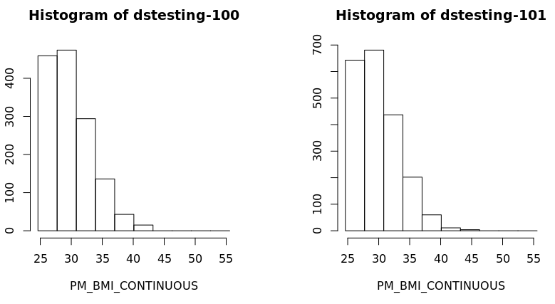
Also a histogram of the variable BMI of the new subset data frame could be created for each study separately:

Div

style	page-break-after:always;

ds.histogram('BMI25plus$PM_BMI_CONTINUOUS', datasources = opals)

Code Block

language	xml

ds.histogram('BMI25plus$PM_BMI_CONTINUOUS', datasources = opals)

Warning: dstesting-100: 2 invalid cells
Warning: dstesting-101: 1 invalid cells
[[1]]
$breaks
 [1] 23.93659 27.17016 30.40373 33.63731 36.87088 40.10445 43.33803 46.57160 49.80518 53.03875 56.27232
$counts
 [1] 365 511 331 150  49  15   0   0   0   0
$density
 [1] 0.079212771 0.110897880 0.071834047 0.032553194 0.010634043 0.003255319 0.000000000 0.000000000 0.000000000 0.000000000
$mids
 [1] 25.55337 28.78695 32.02052 35.25409 38.48767 41.72124 44.95482 48.18839 51.42196 54.65554
$xname
[1] "xvect"
$equidist
[1] TRUE
attr(,"class")
[1] "histogram"

[[2]]
$breaks
 [1] 23.93659 27.17016 30.40373 33.63731 36.87088 40.10445 43.33803 46.57160 49.80518 53.03875 56.27232
$counts
 [1] 506 750 476 229  62  11   4   0   0   0
$density
 [1] 0.0767450721 0.1137525773 0.0721949690 0.0347324536 0.0094035464 0.0016683711 0.0006066804 0.0000000000 0.0000000000 0.0000000000
$mids
 [1] 25.55337 28.78695 32.02052 35.25409 38.48767 41.72124 44.95482 48.18839 51.42196 54.65554
$xname
[1] "xvect"
$equidist
[1] TRUE
attr(,"class")
[1] "histogram

Conclusion

The other parts in this DataSHIELD tutorial series are:

1: Introduction and logging in
2: Basic statistics and data manipulations
3: Assign functions and tables
4: Plotting graphs
5: Subsetting
6: Modelling

Tip

Also remember you can:

get a function list for any DataSHIELD package and
view the manual help page individual functions
in the DataSHIELD test environment it is possible to print analyses to file (.csv, .txt, .pdf, .png)
take a look at our FAQ page for solutions to common problems such as Changing variable class to use in a specific DataSHIELD function.
Get support from our DataSHIELD forum.

...

Versions Compared

Old Version 6

New Version 7

Key

Introduction

Quick reminder for logging in:

Start R/RStudio

Load Packages

Build your login dataframe

Sub-setting

Sub-setting by class

Other general examples of sub-setting

Sub-set by inequality

Sub-setting using ds.subsetByClass

Sub-setting using ds.subset

Conclusion

Page Comparison

Versions Compared

Old Version 6

New Version 7

Key

Introduction

Quick reminder for logging in:

Start R/RStudio

Load Packages

Build your login dataframe

Sub-setting

Sub-setting by class

Other general examples of sub-setting

Sub-set by inequality

Sub-setting using ds.subsetByClass

Sub-setting using ds.subset

Conclusion