Overview
This tutorial demonstrates some of the new functionality and features included in the v5 version of DataSHIELD. We will focus on data manipulation (including dataset sorting and subsetting, data conversion from long to wide and from wide to long formats, merging of datasets, etc), data visualisations (e.g. scatter plots and heatmap plots) and generalised linear model regressions through DataSHIELD.
Before we continue with our session, log onto the DataSHIELD Training Environment
Start the Opal Servers
Your trainer will have started your Opal training servers in the cloud for you.
Logging into the DataSHIELD Client Portal
Your trainer will give you the IP address of the DataSHIELD client portal ending :8787
They will also provide you with a username and password to login with.
Start R/RStudio and load the required packages
| Code Block |
|---|
|
# load libraries
library(opal)
Loading required package: RCurl
Loading required package: bitops
Loading required package: rjson
Loading required package: mime

library(dsBaseClient) |
Part A: Data Manipulation and Data Visualisations
Build your login dataframe and start the Opal Servers
In part A of this demonstration we use the SURVIVAL.EXPAND_WITH_MISSING datasets that include synthetic longitundinal data. Each dataset is in a long format, which means that each row is one time point per subject. So each subject (individual) will have data in multiple rows.
| Code Block |
|---|
| language | bash |
|---|
| title | Build your login dataframe |
|---|
|
server <- c("study1", "study2", "study3") # The VM names
url <- c("http://XXX.XXX.XXX.XXX:8080","http://XXX.XXX.XXX.XXX:8080","http://XXX.XXX.XXX.XXX:8080") # The fixed IP addresses of the training VMs
user <- "administrator"
password <- "datashield_test&"
table <- c("SURVIVAL.EXPAND_WITH_MISSING1","SURVIVAL.EXPAND_WITH_MISSING2","SURVIVAL.EXPAND_WITH_MISSING3") # The data tables used in this tutorial
my_logindata <- data.frame(server,url,user,password,table) |
- The output below indicates that each of the three training datasets
study1, study2 and study3 contain the same variables listed under Variables assigned:
| Code Block |
|---|
| language | bash |
|---|
| title | Build your login dataframe |
|---|
|
> opals <- datashield.login(logins=my_logindata, assign=TRUE)

Logging into the collaborating servers

  No variables have been specified.
  All the variables in the opal table
  (the whole dataset) will be assigned to R!

Assigning data:
study1...
study2...
study3...

Variables assigned:
study1--id, study.id, time.id, starttime, endtime, survtime, cens, age.60, female, noise.56, pm10.16, bmi.26
study2--id, study.id, time.id, starttime, endtime, survtime, cens, age.60, female, noise.56, pm10.16, bmi.26
study3--id, study.id, time.id, starttime, endtime, survtime, cens, age.60, female, noise.56, pm10.16, bmi.26 |
Basic statistics and data manipulations
We can use functions that we have learned in the "Introduction to DataSHIELD" tutorial to get an overview of some characteristics of the three datasets. For example, we can use the ds.dim function to see the dimensions of the datasets and the ds.colnames function to get the names of the variables from each dataset.
| Code Block |
|---|
| language | bash |
|---|
| title | Build your login dataframe |
|---|
|
> ds.dim(x = 'D')
$`dimensions of D in study1`
[1] 2060   12

$`dimensions of D in study2`
[1] 1640   12

$`dimensions of D in study3`
[1] 2688   12

$`dimensions of D in combined studies`
[1] 6388   12

> ds.colnames(x='D', datasources = opals)
$study1
 [1] "id"        "study.id"  "time.id"   "starttime" "endtime"   "survtime"  "cens"      "age.60"    "female"
[10] "noise.56"  "pm10.16"   "bmi.26"

$study2
 [1] "id"        "study.id"  "time.id"   "starttime" "endtime"   "survtime"  "cens"      "age.60"    "female"
[10] "noise.56"  "pm10.16"   "bmi.26"

$study3
 [1] "id"        "study.id"  "time.id"   "starttime" "endtime"   "survtime"  "cens"      "age.60"    "female"
[10] "noise.56" "pm10.16" "bmi.26" |
We can use the ds.reShape function to convert a dataset from long to wide format. In the wide format, a subject’s repeated responses will be in a single row, and each response is in a separate column. The argument timevar.name specifies the column in the long format data that differentiates multiple records from the same subject, and the argument id.var specifies the column that identifies multiple records from the same subject. For more details you can see the function's help file.
...
| Code Block |
|---|
|
> ds.ls()
$study1
[1] "D"      "Dwide1" "Dwide2" "Dwide3"

$study2
[1] "D"      "Dwide1" "Dwide2" "Dwide3"

$study3
[1] "D"      "Dwide1" "Dwide2" "Dwide3"

> ds.colnames('Dwide2')
$study1
 [1] "id"        "study.id"  "starttime" "endtime"   "survtime"  "cens"      "age.60"    "female"    "noise.56"  "pm10.16"
[11] "bmi.26_1"  "bmi.26_4"  "bmi.26_6"  "bmi.26_3"  "bmi.26_2"  "bmi.26_5"

$study2
 [1] "id"        "study.id"  "starttime" "endtime"   "survtime"  "cens"      "age.60"    "female"    "noise.56"  "pm10.16"
[11] "bmi.26_1"  "bmi.26_3"  "bmi.26_2"  "bmi.26_4"  "bmi.26_5"  "bmi.26_6"

$study3
 [1] "id"        "study.id"  "starttime" "endtime"   "survtime"  "cens"      "age.60"    "female"    "noise.56"  "pm10.16"
[11] "bmi.26_1"  "bmi.26_4"  "bmi.26_2"  "bmi.26_3"  "bmi.26_5"  "bmi.26_6"

> ds.colnames('Dwide3')
$study1
 [1] "id"        "study.id"  "cens"      "age.60"    "female"    "noise.56"  "bmi.26"    "pm10.16_1" "pm10.16_4" "pm10.16_6"
[11] "pm10.16_3" "pm10.16_2" "pm10.16_5"

$study2
 [1] "id"        "study.id"  "cens"      "age.60"    "female"    "noise.56"  "bmi.26"    "pm10.16_1" "pm10.16_3" "pm10.16_2"
[11] "pm10.16_4" "pm10.16_5" "pm10.16_6"

$study3
 [1] "id"        "study.id"  "cens"      "age.60"    "female"    "noise.56"  "bmi.26"    "pm10.16_1" "pm10.16_4" "pm10.16_2"
[11] "pm10.16_3" "pm10.16_5" "pm10.16_6" |
Using the same function we can convert a dataset from wide to long format if we set the argument direction to "long". In that case, we have to use the argument varying to specify which variables in the wide format, correspond to single variables in the long format.
...
| Code Block |
|---|
|
> ds.colnames('Dlong2')
$study1
 [1] "id"        "study.id"  "starttime" "endtime"   "survtime"  "cens"      "age.60"    "female"    "noise.56"  "pm10.16"
[11] "time"      "bmi"

$study2
 [1] "id"        "study.id"  "starttime" "endtime"   "survtime"  "cens"      "age.60"    "female"    "noise.56"  "pm10.16"
[11] "time"      "bmi"

$study3
 [1] "id"        "study.id"  "starttime" "endtime"   "survtime"  "cens"      "age.60"    "female"    "noise.56"  "pm10.16"
[11] "time" "bmi" |
Merge data frames
We can use the function ds.merge to merge (link) two data frames together based on common values in vectors defined by the arguments by.x.names and by.y.names.
...
| Code Block |
|---|
|
> ds.colnames("Dwide_merged")
$study1
 [1] "id"         "study.id.x" "starttime"  "endtime"    "survtime"   "cens.x"     "age.60.x"   "female.x"   "noise.56.x"
[10] "pm10.16"    "bmi.26_1"   "bmi.26_4"   "bmi.26_6"   "bmi.26_3"   "bmi.26_2"   "bmi.26_5"   "study.id.y" "cens.y"
[19] "age.60.y"   "female.y"   "noise.56.y" "bmi.26"     "pm10.16_1"  "pm10.16_4"  "pm10.16_6"  "pm10.16_3"  "pm10.16_2"
[28] "pm10.16_5"

$study2
 [1] "id"         "study.id.x" "starttime"  "endtime"    "survtime"   "cens.x"     "age.60.x"   "female.x"   "noise.56.x"
[10] "pm10.16"    "bmi.26_1"   "bmi.26_3"   "bmi.26_2"   "bmi.26_4"   "bmi.26_5"   "bmi.26_6"   "study.id.y" "cens.y"
[19] "age.60.y"   "female.y"   "noise.56.y" "bmi.26"     "pm10.16_1"  "pm10.16_3"  "pm10.16_2"  "pm10.16_4"  "pm10.16_5"
[28] "pm10.16_6"

$study3
 [1] "id"         "study.id.x" "starttime"  "endtime"    "survtime"   "cens.x"     "age.60.x"   "female.x"   "noise.56.x"
[10] "pm10.16"    "bmi.26_1"   "bmi.26_4"   "bmi.26_2"   "bmi.26_3"   "bmi.26_5"   "bmi.26_6"   "study.id.y" "cens.y"
[19] "age.60.y"   "female.y"   "noise.56.y" "bmi.26"     "pm10.16_1"  "pm10.16_4"  "pm10.16_2"  "pm10.16_3"  "pm10.16_5"
[28] "pm10.16_6" |
Dataframe manipulations
Another set of functions that allow data manipulation in DataSHIELD includes the functions ds.dataFrame, ds.dataFrameSort and ds.dataFrameSubset. The ds.dataFrame function creates a data frame from elemental components that can be pre-existing data frames, single variables and/or matrices. The ds.dataFrameSort function sorts a data frame using a specified sort key and the ds.dataFrameSubset function subsets a data frame by row or by column. See the following examples.
...
| Code Block |
|---|
|
> ds.dataFrameSubset(df.name="Dwide2", V1="Dwide2$female", V2="1", Boolean.operator="==", newobj="Dwide2_females")
$is.object.created
[1] "A data object <Dwide2_females> has been created in all specified data sources"

$validity.check
[1] "<Dwide2_females> appears valid in all sources"

> ds.dim("Dwide2")
$`dimensions of Dwide2 in study1`
[1] 886  16

$`dimensions of Dwide2 in study2`
[1] 659  16

$`dimensions of Dwide2 in study3`
[1] 1167   16

$`dimensions of Dwide2 in combined studies`
[1] 2712   16

> ds.dim("Dwide2_females")
$`dimensions of Dwide2_females in study1`
[1] 441  16

$`dimensions of Dwide2_females in study2`
[1] 344  16

$`dimensions of Dwide2_females in study3`
[1] 583  16

$`dimensions of Dwide2_females in combined studies`
[1] 1368 16 |
Data visualisations
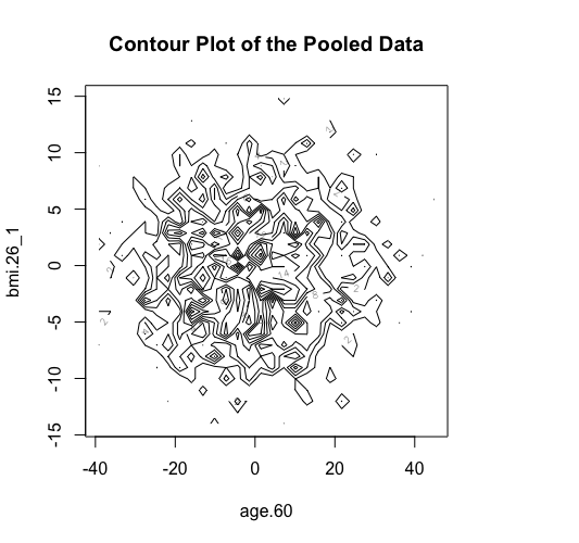
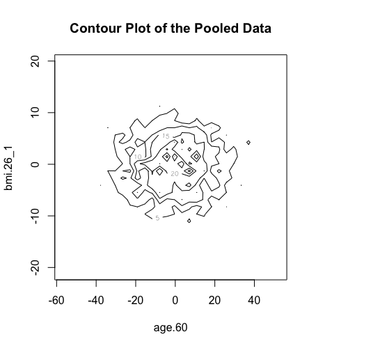
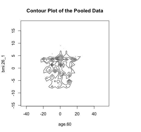
The new ds.scatterPlot function uses two anonymization techniques that produce non-disclosive coordinates that can be displayed in a scatter plot. The anonymization technique is specified by the user in the argument method where there are two possible choices; the "deterministic" and the "probabilistic". If the 'deteministic' method is selected (the default option), then the generated scatter plot shows the scaled centroids of each k nearest neighbours of the original variables where the value of k is set by the user. If the 'probabilistic' method is selected, then the generated scatter plot shows the original data disturbed by the addition of random stochastic noise. The added noise follows a normal distribution with zero mean and variance equal to a percentage of the initial variance of each variable. This percentage is specified by the user in the argument noise.
...
| Code Block |
|---|
| language | bash |
|---|
| title | Build your login dataframe |
|---|
|
> ds.contourPlot(x="Dwide2$age.60", y="Dwide2$bmi.26_1", method="deterministic", noise=3, numints=30)
> ds.contourPlot(x="Dwide2$age.60", y="Dwide2$bmi.26_1", method="probabilistic", noise=0.25, numints=30)
> ds.contourPlot(x="Dwide2$age.60", y="Dwide2$bmi.26_1", method="smallCellsRule", numints=30)
study1: Number of invalid cells (cells with counts >0 and <5) is 261
study2: Number of invalid cells (cells with counts >0 and <5) is 226
study3: Number of invalid cells (cells with counts >0 and <5) is 247 |
Logout the DataSHIELD session
| Code Block |
|---|
| language | bash |
|---|
| title | Build your login dataframe |
|---|
|
> datashield.logout(opals) |
Part B: Generalized Linear Modelling
This part of the tutorial takes you through some of the practicalities and understanding needed to fit a generalized linear model (GLM) in DataSHIELD. To introduce you to a range of different types of regression, the practical works with GLMs fitted using (i) linear ("gaussian") regression; (ii) logistic regression; and (iii) Poisson regression. The linear and logistic regression will both be carried out on a synthetic dataset ("SD") that was initially based upon and generated from the harmonized dataset created and used by the Healthy Obese project (HOP) of the BioSHaRE-eu FP7 project. Metadata about the relatively small number of variables we actually use from SD are generated as the first part of the exercise. Two of the variables generated in the SD dataset denoted a follow-up time (FUT: time in years) and a censoring indicator (cens: 0 = still alive at the end of that follow-up time, 1 = died of any cause at the designated survival time). These variables provide a basis for fitting survival time models. In DataSHIELD at present we enable piecewise exponential regression (PER) to carry out survival analysis - this is a form of Poisson regression and the results it generates are usually very similar to those from Cox regression. The set up and fitting of PER models is explained further below.
Build the login dataframe and start the Opal Servers
| Code Block |
|---|
| language | bash |
|---|
| title | Build your login dataframe |
|---|
|
> server <- c("study1", "study2", "study3") # The VM names
> url <- c("http://XXX.XXX.XXX.XXX:8080","http://XXX.XXX.XXX.XXX:8080","http://XXX.XXX.XXX.XXX:8080")
> user <- "administrator"
> password <- "datashield_test&"
> table <- c("SURVIVAL.COLLAPSE_WITH_MISSING1", "SURVIVAL.COLLAPSE_WITH_MISSING2", "SURVIVAL.COLLAPSE_WITH_MISSING3")
> sd_logindata <- data.frame(server, url, user, password,table)
> opals.sm <- datashield.login(logins=sd_logindata, assign=TRUE, symbol="SD")
Logging into the collaborating servers

  No variables have been specified.
  All the variables in the opal table
  (the whole dataset) will be assigned to R!

Assigning data:
study1...
study2...
study3...

Variables assigned:
study1--ID, STUDY.ID, STARTTIME, ENDTIME, SURVTIME, CENS, age.60, female, noise.56, pm10.16, bmi.26
study2--ID, STUDY.ID, STARTTIME, ENDTIME, SURVTIME, CENS, age.60, female, noise.56, pm10.16, bmi.26
study3--ID, STUDY.ID, STARTTIME, ENDTIME, SURVTIME, CENS, age.60, female, noise.56, pm10.16, bmi.26 |
Create descriptive metadata for the variables to be used in the linear and logistic regression analyses. The outcome variables are the "sbp", a quantitative approximately normally distributed variable denoting measured systolic blood pressure (mm of mercury = mm/Hg [the usual units for BP]) that will be used in the linear regression and "sob", a binary indicator of respiratory dysfunction: 0=no shortness of breath, 1=short of breath, that will be used in the logistic regression.
...
| Code Block |
|---|
| language | bash |
|---|
| title | Build your login dataframe |
|---|
|
ds.scatterPlot(x="age.60", y="age.60.sq") |
Fitting straightforward linear and logistic regression models
1. Fit a conventional multiple linear regression model using sbp as its outcome variable. Start by regressing sbp on female.n and age.60.
...
(Q22) What do you conclude from the coefficients (and standard error) of the interaction term female.E1:bmi.26.E.
Part C: Generalized Linear Modelling with pooling via SLMA using ds.glmSLMA
Under ds.glmSLMA, a glm is fitted to completion at each data source. The estimates and standard errors from each source are then all returned to the client and are combined using study-level meta-analysis. By preference this uses a random effects meta-analysis approach but fixed effects meta-analysis may be used instead.
...