DataSHIELD v5 new functionality
- Data 2 Knowledge
- Alex Westerberg (Unlicensed)
- Hasan Alradhi (Unlicensed)
Bit.ly quick link
Overview
This tutorial demonstrates some of the new functionality and features included in the v5 version of DataSHIELD. We will focus on data manipulation (including dataset sorting and subsetting, data conversion from long to wide and from wide to long formats, merging of datasets, etc), data visualisations (e.g. scatter plots and heatmap plots) and generalised linear model regressions through DataSHIELD.
Before we continue with our session, log onto the DataSHIELD Training Environment
Your trainer will have started your Opal training servers in the cloud for you.
Logging into the DataSHIELD Client Portal
Your trainer will give you the IP address of the DataSHIELD client portal ending :8787
They will also provide you with a username and password to login with.
Start R/RStudio and load the required packages
# load libraries
library(opal)
Loading required package: RCurl
Loading required package: bitops
Loading required package: rjson
Loading required package: mime

library(dsBaseClient)
Part A: Data Manipulation and Data Visualisations
> opals <- datashield.login(logins=my_logindata, assign=TRUE)

Logging into the collaborating servers

  No variables have been specified.
  All the variables in the opal table
  (the whole dataset) will be assigned to R!

Assigning data:
study1...
study2...
study3...

Variables assigned:
study1--id, study.id, time.id, starttime, endtime, survtime, cens, age.60, female, noise.56, pm10.16, bmi.26
study2--id, study.id, time.id, starttime, endtime, survtime, cens, age.60, female, noise.56, pm10.16, bmi.26
study3--id, study.id, time.id, starttime, endtime, survtime, cens, age.60, female, noise.56, pm10.16, bmi.26
Basic statistics and data manipulations
We can use functions that we have learned in the "Introduction to DataSHIELD" tutorial to get an overview of some characteristics of the three datasets. For example, we can use the ds.dim function to see the dimensions of the datasets and the ds.colnames function to get the names of the variables from each dataset.
> ds.dim(x = 'D')
$`dimensions of D in study1`
[1] 2060   12

$`dimensions of D in study2`
[1] 1640   12

$`dimensions of D in study3`
[1] 2688   12

$`dimensions of D in combined studies`
[1] 6388   12

> ds.colnames(x='D', datasources = opals)
$study1
 [1] "id"        "study.id"  "time.id"   "starttime" "endtime"   "survtime"  "cens"      "age.60"    "female"
[10] "noise.56"  "pm10.16"   "bmi.26"

$study2
 [1] "id"        "study.id"  "time.id"   "starttime" "endtime"   "survtime"  "cens"      "age.60"    "female"
[10] "noise.56"  "pm10.16"   "bmi.26"

$study3
 [1] "id"        "study.id"  "time.id"   "starttime" "endtime"   "survtime"  "cens"      "age.60"    "female"
[10] "noise.56"  "pm10.16"   "bmi.26"
Reshape from long to wide format
We can use the ds.reShape function to convert a dataset from long to wide format. In the wide format, a subject’s repeated responses will be in a single row, and each response is in a separate column. The argument timevar.name specifies the column in the long format data that differentiates multiple records from the same subject, and the argument id.var specifies the column that identifies multiple records from the same subject. For more details you can see the function's help file.
> ds.reShape(data.name='D', timevar.name='time.id', idvar.name='id', direction='wide', newobj="Dwide1", datasources=opals)
$is.object.created
[1] "A data object <Dwide1> has been created in all specified data sources"

$validity.check
[1] "<Dwide1> appears valid in all sources"

> ds.ls()
$study1
[1] "D"      "Dwide1"

$study2
[1] "D"      "Dwide1"

$study3
[1] "D"      "Dwide1"

> ds.dim('Dwide1')
$`dimensions of Dwide1 in study1`
[1] 886  61

$`dimensions of Dwide1 in study2`
[1] 659  61

$`dimensions of Dwide1 in study3`
[1] 1167   61

$`dimensions of Dwide1 in combined studies`
[1] 2712   61
> ds.colnames('Dwide1')
$study1
 [1] "id"          "study.id.1"  "starttime.1" "endtime.1"   "survtime.1"  "cens.1"      "age.60.1"
 [8] "female.1"    "noise.56.1"  "pm10.16.1"   "bmi.26.1"    "study.id.4"  "starttime.4" "endtime.4"
[15] "survtime.4"  "cens.4"      "age.60.4"    "female.4"    "noise.56.4"  "pm10.16.4"   "bmi.26.4"
[22] "study.id.6"  "starttime.6" "endtime.6"   "survtime.6"  "cens.6"      "age.60.6"    "female.6"
[29] "noise.56.6"  "pm10.16.6"   "bmi.26.6"    "study.id.3"  "starttime.3" "endtime.3"   "survtime.3"
[36] "cens.3"      "age.60.3"    "female.3"    "noise.56.3"  "pm10.16.3"   "bmi.26.3"    "study.id.2"
[43] "starttime.2" "endtime.2"   "survtime.2"  "cens.2"      "age.60.2"    "female.2"    "noise.56.2"
[50] "pm10.16.2"   "bmi.26.2"    "study.id.5"  "starttime.5" "endtime.5"   "survtime.5"  "cens.5"
[57] "age.60.5"    "female.5"    "noise.56.5"  "pm10.16.5"   "bmi.26.5"
$study2
 [1] "id"          "study.id.1"  "starttime.1" "endtime.1"   "survtime.1"  "cens.1"      "age.60.1"
 [8] "female.1"    "noise.56.1"  "pm10.16.1"   "bmi.26.1"    "study.id.3"  "starttime.3" "endtime.3"
[15] "survtime.3"  "cens.3"      "age.60.3"    "female.3"    "noise.56.3"  "pm10.16.3"   "bmi.26.3"
[22] "study.id.2"  "starttime.2" "endtime.2"   "survtime.2"  "cens.2"      "age.60.2"    "female.2"
[29] "noise.56.2"  "pm10.16.2"   "bmi.26.2"    "study.id.4"  "starttime.4" "endtime.4"   "survtime.4"
[36] "cens.4"      "age.60.4"    "female.4"    "noise.56.4"  "pm10.16.4"   "bmi.26.4"    "study.id.5"
[43] "starttime.5" "endtime.5"   "survtime.5"  "cens.5"      "age.60.5"    "female.5"    "noise.56.5"
[50] "pm10.16.5"   "bmi.26.5"    "study.id.6"  "starttime.6" "endtime.6"   "survtime.6"  "cens.6"
[57] "age.60.6"    "female.6"    "noise.56.6"  "pm10.16.6"   "bmi.26.6"
$study3
 [1] "id"          "study.id.1"  "starttime.1" "endtime.1"   "survtime.1"  "cens.1"      "age.60.1"
 [8] "female.1"    "noise.56.1"  "pm10.16.1"   "bmi.26.1"    "study.id.4"  "starttime.4" "endtime.4"
[15] "survtime.4"  "cens.4"      "age.60.4"    "female.4"    "noise.56.4"  "pm10.16.4"   "bmi.26.4"
[22] "study.id.2"  "starttime.2" "endtime.2"   "survtime.2"  "cens.2"      "age.60.2"    "female.2"
[29] "noise.56.2"  "pm10.16.2"   "bmi.26.2"    "study.id.3"  "starttime.3" "endtime.3"   "survtime.3"
[36] "cens.3"      "age.60.3"    "female.3"    "noise.56.3"  "pm10.16.3"   "bmi.26.3"    "study.id.5"
[43] "starttime.5" "endtime.5"   "survtime.5"  "cens.5"      "age.60.5"    "female.5"    "noise.56.5"
[50] "pm10.16.5"   "bmi.26.5"    "study.id.6"  "starttime.6" "endtime.6"   "survtime.6"  "cens.6"
[57] "age.60.6"    "female.6"    "noise.56.6"  "pm10.16.6"   "bmi.26.6"
We can also choose for which variables to create multiple columns depending on the time.var by using the argument v.names and also we can use the argument drop if we want to drop some of the variables in the wide format.
> ds.reShape(data.name='D', v.names='bmi.26', timevar.name='time.id', idvar.name='id', direction='wide', newobj="Dwide2", datasources=opals, sep='_')
$is.object.created
[1] "A data object <Dwide2> has been created in all specified data sources"

$validity.check
[1] "<Dwide2> appears valid in all sources"
> ds.reShape(data.name='D', v.names='pm10.16', timevar.name='time.id', idvar.name='id', direction='wide', newobj="Dwide3", datasources=opals, sep='_', drop=c('starttime','endtime','survtime'))
$is.object.created
[1] "A data object <Dwide3> has been created in all specified data sources"

$validity.check
[1] "<Dwide3> appears valid in all sources"
> ds.ls()
$study1
[1] "D"      "Dwide1" "Dwide2" "Dwide3"

$study2
[1] "D"      "Dwide1" "Dwide2" "Dwide3"

$study3
[1] "D"      "Dwide1" "Dwide2" "Dwide3"

> ds.colnames('Dwide2')
$study1
 [1] "id"        "study.id"  "starttime" "endtime"   "survtime"  "cens"      "age.60"    "female"    "noise.56"  "pm10.16"
[11] "bmi.26_1"  "bmi.26_4"  "bmi.26_6"  "bmi.26_3"  "bmi.26_2"  "bmi.26_5"

$study2
 [1] "id"        "study.id"  "starttime" "endtime"   "survtime"  "cens"      "age.60"    "female"    "noise.56"  "pm10.16"
[11] "bmi.26_1"  "bmi.26_3"  "bmi.26_2"  "bmi.26_4"  "bmi.26_5"  "bmi.26_6"

$study3
 [1] "id"        "study.id"  "starttime" "endtime"   "survtime"  "cens"      "age.60"    "female"    "noise.56"  "pm10.16"
[11] "bmi.26_1"  "bmi.26_4"  "bmi.26_2"  "bmi.26_3"  "bmi.26_5"  "bmi.26_6"

> ds.colnames('Dwide3')
$study1
 [1] "id"        "study.id"  "cens"      "age.60"    "female"    "noise.56"  "bmi.26"    "pm10.16_1" "pm10.16_4" "pm10.16_6"
[11] "pm10.16_3" "pm10.16_2" "pm10.16_5"

$study2
 [1] "id"        "study.id"  "cens"      "age.60"    "female"    "noise.56"  "bmi.26"    "pm10.16_1" "pm10.16_3" "pm10.16_2"
[11] "pm10.16_4" "pm10.16_5" "pm10.16_6"

$study3
 [1] "id"        "study.id"  "cens"      "age.60"    "female"    "noise.56"  "bmi.26"    "pm10.16_1" "pm10.16_4" "pm10.16_2"
[11] "pm10.16_3" "pm10.16_5" "pm10.16_6"
Reshape from wide to long format
Using the same function we can convert a dataset from wide to long format if we set the argument direction to "long". In that case, we have to use the argument varying to specify which variables in the wide format, correspond to single variables in the long format.
> ds.reShape(data.name='Dwide2', varying=list("bmi.26_1", "bmi.26_3", "bmi.26_2", "bmi.26_4", "bmi.26_5", "bmi.26_6"), direction='long', newobj="Dlong2", datasources=opals)
$is.object.created
[1] "A data object <Dlong2> has been created in all specified data sources"

$validity.check
[1] "<Dlong2> appears valid in all sources"
> ds.ls()
$study1
[1] "D"      "Dlong2" "Dwide1" "Dwide2" "Dwide3"

$study2
[1] "D"      "Dlong2" "Dwide1" "Dwide2" "Dwide3"

$study3
[1] "D"      "Dlong2" "Dwide1" "Dwide2" "Dwide3"

> ds.dim('Dlong2')
$`dimensions of Dlong2 in study1`
[1] 5316   12

$`dimensions of Dlong2 in study2`
[1] 3954   12

$`dimensions of Dlong2 in study3`
[1] 7002   12

$`dimensions of Dlong2 in combined studies`
[1] 16272    12
> ds.colnames('Dlong2')
$study1
 [1] "id"        "study.id"  "starttime" "endtime"   "survtime"  "cens"      "age.60"    "female"    "noise.56"  "pm10.16"
[11] "time"      "bmi"

$study2
 [1] "id"        "study.id"  "starttime" "endtime"   "survtime"  "cens"      "age.60"    "female"    "noise.56"  "pm10.16"
[11] "time"      "bmi"

$study3
 [1] "id"        "study.id"  "starttime" "endtime"   "survtime"  "cens"      "age.60"    "female"    "noise.56"  "pm10.16"
[11] "time"      "bmi"
Merge data frames
We can use the function ds.merge to merge (link) two data frames together based on common values in vectors defined by the arguments by.x.names and by.y.names.
> ds.merge(x.name="Dwide2", y.name="Dwide3", by.x.names="id", by.y.names="id", sort=TRUE, newobj="Dwide_merged", datasources=opals)
$is.object.created
[1] "A data object <Dwide_merged> has been created in all specified data sources"

$validity.check
[1] "<Dwide_merged> appears valid in all sources"

> ds.ls()
$study1
[1] "D"            "Dlong2"       "Dwide1"       "Dwide2"       "Dwide3"       "Dwide_merged"

$study2
[1] "D"            "Dlong2"       "Dwide1"       "Dwide2"       "Dwide3"       "Dwide_merged"

$study3
[1] "D"            "Dlong2"       "Dwide1"       "Dwide2"       "Dwide3"       "Dwide_merged"
> ds.colnames("Dwide_merged")
$study1
 [1] "id"         "study.id.x" "starttime"  "endtime"    "survtime"   "cens.x"     "age.60.x"   "female.x"   "noise.56.x"
[10] "pm10.16"    "bmi.26_1"   "bmi.26_4"   "bmi.26_6"   "bmi.26_3"   "bmi.26_2"   "bmi.26_5"   "study.id.y" "cens.y"
[19] "age.60.y"   "female.y"   "noise.56.y" "bmi.26"     "pm10.16_1"  "pm10.16_4"  "pm10.16_6"  "pm10.16_3"  "pm10.16_2"
[28] "pm10.16_5"

$study2
 [1] "id"         "study.id.x" "starttime"  "endtime"    "survtime"   "cens.x"     "age.60.x"   "female.x"   "noise.56.x"
[10] "pm10.16"    "bmi.26_1"   "bmi.26_3"   "bmi.26_2"   "bmi.26_4"   "bmi.26_5"   "bmi.26_6"   "study.id.y" "cens.y"
[19] "age.60.y"   "female.y"   "noise.56.y" "bmi.26"     "pm10.16_1"  "pm10.16_3"  "pm10.16_2"  "pm10.16_4"  "pm10.16_5"
[28] "pm10.16_6"

$study3
 [1] "id"         "study.id.x" "starttime"  "endtime"    "survtime"   "cens.x"     "age.60.x"   "female.x"   "noise.56.x"
[10] "pm10.16"    "bmi.26_1"   "bmi.26_4"   "bmi.26_2"   "bmi.26_3"   "bmi.26_5"   "bmi.26_6"   "study.id.y" "cens.y"
[19] "age.60.y"   "female.y"   "noise.56.y" "bmi.26"     "pm10.16_1"  "pm10.16_4"  "pm10.16_2"  "pm10.16_3"  "pm10.16_5"
[28] "pm10.16_6"
Dataframe manipulations
Another set of functions that allow data manipulation in DataSHIELD includes the functions ds.dataFrame, ds.dataFrameSort and ds.dataFrameSubset. The ds.dataFrame function creates a data frame from elemental components that can be pre-existing data frames, single variables and/or matrices. The ds.dataFrameSort function sorts a data frame using a specified sort key and the ds.dataFrameSubset function subsets a data frame by row or by column. See the following examples.
- We can create a dataframe with only complete cases (i.e. the records in each row of a dataframe do not have any missing values).
> ds.dim('D')
$`dimensions of D in study1`
[1] 2060   12

$`dimensions of D in study2`
[1] 1640   12

$`dimensions of D in study3`
[1] 2688   12

$`dimensions of D in combined studies`
[1] 6388   12
> ds.dim('Dlong2')
$`dimensions of Dlong2 in study1`
[1] 5316   12

$`dimensions of Dlong2 in study2`
[1] 3954   12

$`dimensions of Dlong2 in study3`
[1] 7002   12

$`dimensions of Dlong2 in combined studies`
[1] 16272    12

> ds.dataFrame(x='D', completeCases=TRUE, newobj='Db')
$is.object.created
[1] "A data object <Db> has been created in all specified data sources"

$validity.check
[1] "<Db> appears valid in all sources"

> ds.dataFrame(x='Dlong2', completeCases=TRUE, newobj='Dlong2b')
$is.object.created
[1] "A data object <Dlong2b> has been created in all specified data sources"

$validity.check
[1] "<Dlong2b> appears valid in all sources"
> ds.dim('Db')
$`dimensions of Db in study1`
[1] 1974   12

$`dimensions of Db in study2`
[1] 1528   12

$`dimensions of Db in study3`
[1] 2529   12

$`dimensions of Db in combined studies`
[1] 6031   12

> ds.dim('Dlong2b')
$`dimensions of Dlong2b in study1`
[1] 1974   12

$`dimensions of Dlong2b in study2`
[1] 1528   12

$`dimensions of Dlong2b in study3`
[1] 2529   12

$`dimensions of Dlong2b in combined studies`
[1] 6031   12
- We can create a subset of a dataframe based on a binary variable.
> ds.table1D(x="Dwide2$female")
$counts
      Dwide2$female
0              1324
1              1368
Total          2692

$percentages
      Dwide2$female
0             49.18
1             50.82
Total        100.00

$validity
[1] "All tables are valid!"
> ds.dataFrameSubset(df.name="Dwide2", V1="Dwide2$female", V2="1", Boolean.operator="==", newobj="Dwide2_females")
$is.object.created
[1] "A data object <Dwide2_females> has been created in all specified data sources"

$validity.check
[1] "<Dwide2_females> appears valid in all sources"

> ds.dim("Dwide2")
$`dimensions of Dwide2 in study1`
[1] 886  16

$`dimensions of Dwide2 in study2`
[1] 659  16

$`dimensions of Dwide2 in study3`
[1] 1167   16

$`dimensions of Dwide2 in combined studies`
[1] 2712   16

> ds.dim("Dwide2_females")
$`dimensions of Dwide2_females in study1`
[1] 441  16

$`dimensions of Dwide2_females in study2`
[1] 344  16

$`dimensions of Dwide2_females in study3`
[1] 583  16

$`dimensions of Dwide2_females in combined studies`
[1] 1368   16
Data visualisations
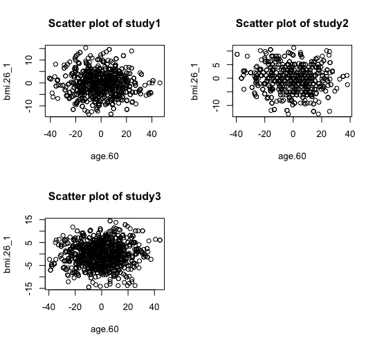
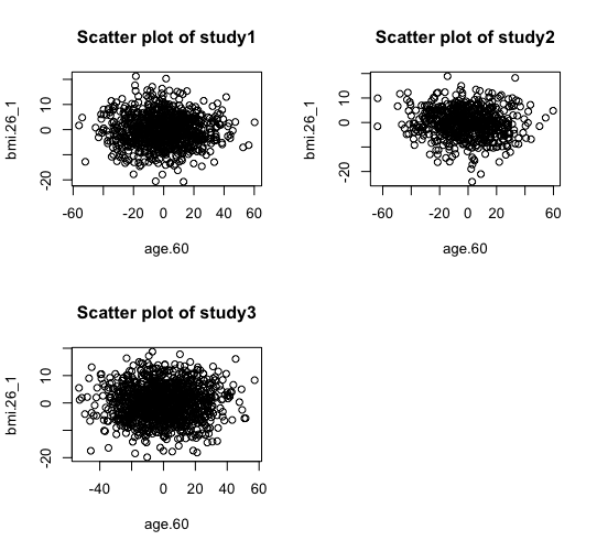
The new ds.scatterPlot function uses two anonymization techniques that produce non-disclosive coordinates that can be displayed in a scatter plot. The anonymization technique is specified by the user in the argument method where there are two possible choices; the "deterministic" and the "probabilistic". If the 'deteministic' method is selected (the default option), then the generated scatter plot shows the scaled centroids of each k nearest neighbours of the original variables where the value of k is set by the user. If the 'probabilistic' method is selected, then the generated scatter plot shows the original data disturbed by the addition of random stochastic noise. The added noise follows a normal distribution with zero mean and variance equal to a percentage of the initial variance of each variable. This percentage is specified by the user in the argument noise.
> ds.scatterPlot(x="Dwide2$age.60", y="Dwide2$bmi.26_1", method="deterministic", k=3)
[1] "Split plot created"
> ds.scatterPlot(x="Dwide2$age.60", y="Dwide2$bmi.26_1", method="probabilistic", noise=0.5)
[1] "Split plot created"
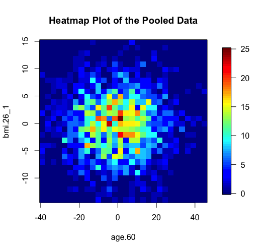
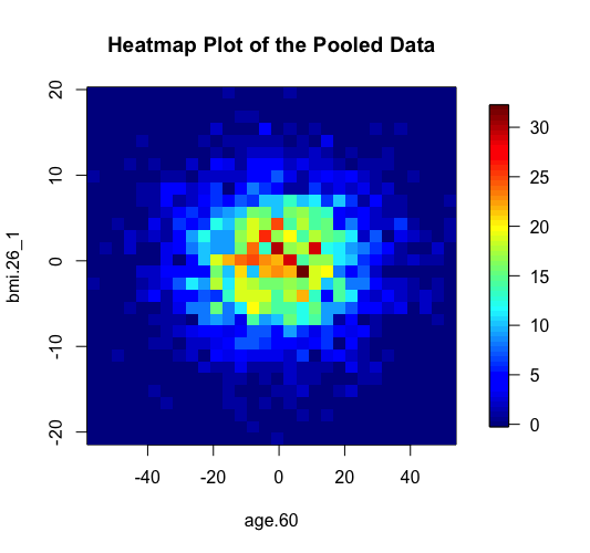
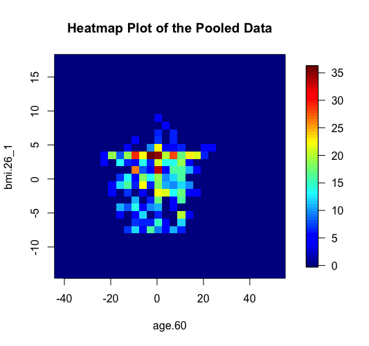
The same two methods of anonymisation (i.e. the deterministic and probabilistic) have been added as additional options in the previously existing graphical functions of DataSHIELD including the functions ds.histogram, ds.heatmapPlot and ds.contourPlot. In the example below we can see the behavior of the two methods in the generation of non-disclosive heatmap plots (left and middle panels) and compare them with the previously existing method of small cells suppression rule (right panel) where grids with small density (smaller than a pre-specified filter) are suppresed from the density grid matrix (i.e. their values replaced by zeros). If the user selects the "smallCellsRule" method, then the function returns the number of invalid cells from each study.
> ds.heatmapPlot(x="Dwide2$age.60", y="Dwide2$bmi.26_1", method="deterministic", noise=3, numints=30)
> ds.heatmapPlot(x="Dwide2$age.60", y="Dwide2$bmi.26_1", method="probabilistic", noise=0.25, numints=30)
> ds.heatmapPlot(x="Dwide2$age.60", y="Dwide2$bmi.26_1", method="smallCellsRule", numints=30)
study1: Number of invalid cells (cells with counts >0 and <5) is 261
study2: Number of invalid cells (cells with counts >0 and <5) is 226
study3: Number of invalid cells (cells with counts >0 and <5) is 247
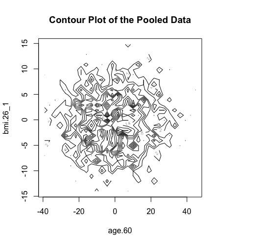
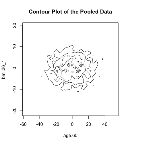
We can do similar observations with the generation of contour plots using the function ds.contourPlot.
> ds.contourPlot(x="Dwide2$age.60", y="Dwide2$bmi.26_1", method="deterministic", noise=3, numints=30)
> ds.contourPlot(x="Dwide2$age.60", y="Dwide2$bmi.26_1", method="probabilistic", noise=0.25, numints=30)
> ds.contourPlot(x="Dwide2$age.60", y="Dwide2$bmi.26_1", method="smallCellsRule", numints=30)
study1: Number of invalid cells (cells with counts >0 and <5) is 261
study2: Number of invalid cells (cells with counts >0 and <5) is 226
study3: Number of invalid cells (cells with counts >0 and <5) is 247

Logout the DataSHIELD session
> datashield.logout(opals)
Part B: Generalized Linear Modelling
This part of the tutorial takes you through some of the practicalities and understanding needed to fit a generalized linear model (GLM) in DataSHIELD. To introduce you to a range of different types of regression, the practical works with GLMs fitted using (i) linear ("gaussian") regression; (ii) logistic regression; and (iii) Poisson regression. The linear and logistic regression will both be carried out on a synthetic dataset ("SD") that was initially based upon and generated from the harmonized dataset created and used by the Healthy Obese project (HOP) of the BioSHaRE-eu FP7 project. Metadata about the relatively small number of variables we actually use from SD are generated as the first part of the exercise. Two of the variables generated in the SD dataset denoted a follow-up time (FUT: time in years) and a censoring indicator (cens: 0 = still alive at the end of that follow-up time, 1 = died of any cause at the designated survival time). These variables provide a basis for fitting survival time models. In DataSHIELD at present we enable piecewise exponential regression (PER) to carry out survival analysis - this is a form of Poisson regression and the results it generates are usually very similar to those from Cox regression. The set up and fitting of PER models is explained further below.
Build the login dataframe and start the Opal Servers
> server <- c("study1", "study2", "study3") # The VM names
> url <- c("http://XXX.XXX.XXX.XXX:8080","http://XXX.XXX.XXX.XXX:8080","http://XXX.XXX.XXX.XXX:8080")
> user <- "administrator"
> password <- "datashield_test&"
> table <- c("SURVIVAL.COLLAPSE_WITH_MISSING1", "SURVIVAL.COLLAPSE_WITH_MISSING2", "SURVIVAL.COLLAPSE_WITH_MISSING3")
> sd_logindata <- data.frame(server, url, user, password,table)
> opals.sm <- datashield.login(logins=sd_logindata, assign=TRUE, symbol="SD")
Logging into the collaborating servers

  No variables have been specified.
  All the variables in the opal table
  (the whole dataset) will be assigned to R!

Assigning data:
study1...
study2...
study3...

Variables assigned:
study1--ID, STUDY.ID, STARTTIME, ENDTIME, SURVTIME, CENS, age.60, female, noise.56, pm10.16, bmi.26
study2--ID, STUDY.ID, STARTTIME, ENDTIME, SURVTIME, CENS, age.60, female, noise.56, pm10.16, bmi.26
study3--ID, STUDY.ID, STARTTIME, ENDTIME, SURVTIME, CENS, age.60, female, noise.56, pm10.16, bmi.26
Simple descriptive metadata
Create descriptive metadata for the variables to be used in the linear and logistic regression analyses. The outcome variables are the "sbp", a quantitative approximately normally distributed variable denoting measured systolic blood pressure (mm of mercury = mm/Hg [the usual units for BP]) that will be used in the linear regression and "sob", a binary indicator of respiratory dysfunction: 0=no shortness of breath, 1=short of breath, that will be used in the logistic regression.
The following code generates useful descriptive statistics for each variable
ds.length("sbp")
ds.class("sbp")
ds.quantileMean("sbp", "split")
ds.histogram("sbp")

ds.length("sob")
ds.class("sob")
ds.table1D("sob", "split")
Explanatory variables:
- female = binary sex indicator in the form of a factor i.e. two levels: level 0 = male, level 1 = female
ds.length("female")
ds.class("female")
ds.table1D("female", "split")
- Coerce female to class numeric (female.n) this leaves the 0s and 1s of female unchanged but R treats female.n as a continuous variable with values that happen to be either 0 and 1
ds.length("female.n")
ds.class("female.n")
ds.histogram("female.n")
ds.table1D("female.n", "split")
- age.60 = age in years minus 60 years - this is approximately normal and by substracting 60, which is close to the mean age, age.60 has a mean close to zero
ds.length("age.60")
ds.class("age.60")
ds.histogram("age.60")
- create variable age.60 squared
ds.make("age.60*age.60", "age.60.sq")
ds.length("age.60.sq")
ds.class("age.60.sq")
ds.histogram("age.60.sq")
- bmi.26 = body mass index (Kg/m2) minus 26
ds.length("bmi.26")
ds.class("bmi.26")
ds.histogram("bmi.26")
- check age.60.sq created correctly? Is the scatter plot as would be expected?
ds.scatterPlot(x="age.60", y="age.60.sq")
Fitting straightforward linear and logistic regression models
1. Fit a conventional multiple linear regression model using sbp as its outcome variable. Start by regressing sbp on female.n and age.60.
ds.glm("sbp~female.n+age.60", family="gaussian")
Use this glm to answer these questions:
(Q1) Are females estimated to have a higher or lower sbp than males?
(Q2) What is the estimated difference in systolic BP between men and women?
(Q3) What its 95% confidence interval (CI)?
(Q4) Having adjusted for the effect of gender by how much is sbp estimated to rise for a 1 year increase in age (with 95% CI)
By changing the arguments to the call to ds.glm estimate the corresponding 99% confidence interval
ds.glm("sbp~female.n+age.60", family="gaussian", CI=0.99)
(Q5) What is the vaue of this 99% CI?
2. Now extend the model to allow the effect of age.60 to be non-linear by adding age.60.sq and also adding bmi.26 to estimate the effect of bmi.26 on sbp having adjusted for gender and age
ds.glm("sbp~female.n+age.60+age.60.sq+bmi.26", family="gaussian")
(Q6) Use the z-value and p-value columns of the coefficients output to determine whether there is "significant" evidence that the effect of age is non-linear. Does the term for non-linearity lead to a significant improvement in model fit?
(Q7) What other test of statistical significance is commonly used in glms? If you wish carry out the relevant likelihood test here. Why do you have to be very careful about the number of missing observations if you use it?
ds.glm("sbp~female.n+age.60+bmi.26", family="gaussian")
(Q8) To demonstrate to non-experts what the modelled relationship of sbp vs age looks like you can use the model including age.60.sq to quantify the relationship:
Create an age.60 variable for a plot across a range covering most of the observed data:
age.60.plot<-(-40:40)
Now use coefficients for constant, age.60 and age.60.sq from the model including age.60.sq to calculate expected value for sbp using that model. Does this look approximately linear?
sbp.plot<-140.0733+1.002158*age.60.plot-0.000144103*(age.60.plot^2)
plot(age.60.plot,sbp.plot)
3. Now fit a logistic regression model using sob as its outcome variable. Start by regressing sob on female.n, age.60 and bmi.26
ds.glm("sob~1+female.n+age.60+bmi.26", family="binomial")
(Q9) Are females are more or less likely to have sob than males?
(Q10) What is the estimated odds ratio (with 95%) confidence interval that quantifies your answer to Q9?
Now fit the same model but print out the variance-covariance and correlation matrices for the parameter (coefficient) estimates. Justlook at these: $VarCovMatrix and $CorrMatrix in case you ever need to use them.
ds.glm("sob~1+female.n+age.60+bmi.26", family="binomial",
       viewVarCov = TRUE, viewCor = TRUE)
Now fit the same model but just for studies 1 and 3
ds.glm("sob~1+female.n+age.60+bmi.26", family="binomial", datasources=opals.sm[c(1,3)])
Fit the same model again - across all studies - but add the variable weights4 as a regression weight. weights4 is a vector of the same length as sob but all elements = 4.
ds.glm("sob~1+female.n+age.60+bmi.26", family="binomial", weights="weights4")
(Q11) What has happened to the coefficient estimates and what has happened to their standard errors? Why has this happened?
4. Now we'll look at some "tricks" in the way you specify the components of a GLM so they make it easier to get out the particular answers you want. So we'll return to the spb models because it is generally easier to interpret linear regression models but everything below applies to other GLMs too.
Regress sbp on female.n and age.60 again:
ds.glm("sbp~female.n+age.60", family="gaussian")
Now replace female.n by female (the factor) and force the glm to fit a constant term (also sometimes called an intercept, grand-mean or corner terms) by putting +1 in the regression formula:
ds.glm("sbp~1+female+age.60", family="gaussian")
The only visible change is that the female.n covariate is now referred to as female1. This formally means level 1 of the female factor (i.e. female in contrast to male).
(Q12) What does the regression constant (140.079) mean?
(Q13) What is the expected sbp in a female at age 60?
Now for our first "trick". Force glm to remove the regression constant:
ds.glm("sbp~female+age.60-1", family="gaussian")

OR

ds.glm("sbp~0+female+age.60", family="gaussian")
(Q14) What do the first two terms now measure?
Now add bmi.26 to the model:
ds.glm("sbp~0+female+age.60+bmi.26", family="gaussian")
(Q15) What does the coefficient for age.60 estimate?
(Q16) What estimate does this model provide for the estimated increase in sbp if age increases by 10 years? What is the standard error of this increase?
Now add an interaction between female and age.60:
ds.glm("sbp~female*age.60+bmi.26", family="gaussian")
(Q17) What does the coefficient for age.60 now estimate? What does the sum of the coefficient for age.60 and the coefficient for the interaction (female1:age.60) measure?
Now for another "trick" in specifying the regression formula. Let us specifically remove the main effect for age.60.
ds.glm("sbp~female*age.60+bmi.26-age.60", family="gaussian")
(Q18) What do the two coefficients asociated with the interaction terms now measure?
5. Now let's fit a Piecewise Exponential Regression (PER) model. The variables we need/can use to create and fit a PER include:
The first step in setting up a piecewise exponential model is to divide the observed survival time into a series of pre-defined time epochs using a DataSHIELD function called ds.lexis. This is a particularly complicated function that we will make no attempt to explain in this practical - but the SD Dataset has been pre-processed using ds.lexis so that a set of variables needed for piecewise exponential regression has already been created as part of an "expanded" dataset in which each row of SD has been replaced by up to 6 rows that are each the same as the row in SD except that the survival time has been split into 6 different periods: 0-2 yrs; 2-3 yrs; 3-6 yrs; 6-6.5 yrs; 6.5-8 yrs; 8-10 yrs. No survival or follow-up time in the SD dataset exceeded 10 yrs. The censoring indicator (died) in each time period took the value 1 if an individual died in that period and 0 if they survived the whole period or their follow-up terminated in that period without them having died.
To illustrate, if in the orginal SD dataset:
FUT=3.47 and cens=0: there will be three rows in the expanded dataset with "survtime" (the length of the follow-up in each period) taking the values 2, 1, 0.47 and "died" taking values 0, 0, 0
FUT=7.83 and cens=1: there will be five rows in the expanded dataset with survtime taking the values 2, 1, 3, 0.5, 1.33 and died taking values 0, 0, 0, 0, 1
FUT=10.0 and cens= 0 (survived for the whole study): there will be six rows with survtime taking the values 2, 1, 3, 0.5, 1.5, 2 and died taking the values 0, 0, 0, 0, 0, 0
Without going into further details, the descriptive metadata for the variables that are needed or could be used in the PER modelling can be generated below:
#survtime
ds.length("survtime")
ds.class("survtime")
ds.histogram("survtime")
ds.quantileMean("survtime", "split")

#died
ds.length("died")
ds.class("died")
ds.histogram("died")
ds.table1D("died", "split")
tid.f this is a factor with levels 1 to 6 which identifies which exposure period each row of the expanded data set relates to. So if tid.f = 2, the row in which it falls will include the values of "died" and "survtime" that apply to the relevant individual during time period 2 (i.e. 2-3 years [see above])
ds.length("tid.f")
ds.class("tid.f")
ds.table1D("tid.f", "split")
female.E this takes the "female" factor using the same value in each row in the SD database expanded to all the corresponding rows in the expanded database created by ds.lexis
ds.length("female.E")
ds.class("female.E")
ds.table1D("female.E", "split")
age.60.E this takes the "age.60" variable using the same value in each row in the SD database expanded to all the corresponding rows in the expanded database created by ds.lexis
ds.length("age.60.E")
ds.class("age.60.E")
ds.histogram("age.60.E")
ds.quantileMean("age.60.E", "split")
bmi.26.E this takes the "bmi.26" variable using the same value in each row in the SD database expanded to all the corresponding rows in the expanded database created by ds.lexis
ds.length("bmi.26.E")
ds.class("bmi.26.E")
ds.histogram("bmi.26.E")
ds.quantileMean("bmi.26.E", "split")
Fit a basic PER model to regress outcome (death or survival) on female.E and age.60.E
First create an offset variable equal to log of survtime:
ds.make("log(survtime)", "log.surv")
ds.histogram("log.surv")
Now specify the model:
ds.glm("died~female.E+age.60.E", family="poisson", offset="log.surv")
(Q19) Why does this specification of the model fit what you need? This question is difficult, but the ideal answer is hopefully useful even if you can't come up with that answer yourself.
Now add tid.f to the regression formula and remove the constant:
ds.glm("died~0+tid.f+female.E+age.60.E", family="poisson", offset="log.surv")
(Q20) What do the coefficients for tid.f now estimate?
(Q21) Just to try fitting a PER model yourself add bmi.26.E to the PER model and enable estimation of the variance-covariance matrix and the correlation matrix of parameter estimates. Is there a significant association of bmi with the risk of death, if so does it increase the risk or decrease it, and by how much?
ds.glm("died~0+tid.f+female.E+bmi.26.E+age.60.E", family="poisson", offset="log.surv",
        viewVarCov = TRUE, viewCor = TRUE)
Now add an interaction between female.E and bmi.26.E
ds.glm("died~0+tid.f+female.E*bmi.26.E+age.60.E", family="poisson", offset="log.surv")
(Q22) What do you conclude from the coefficients (and standard error) of the interaction term female.E1:bmi.26.E.
Part C: Generalized Linear Modelling with pooling via SLMA using ds.glmSLMA
Under ds.glmSLMA, a glm is fitted to completion at each data source. The estimates and standard errors from each source are then all returned to the client and are combined using study-level meta-analysis. By preference this uses a random effects meta-analysis approach but fixed effects meta-analysis may be used instead.
First we'll take the following model fitted under ds.glm and fit it again using ds.glmSLMA:
ds.glm("sbp~female.n+age.60+bmi.26",family="gaussian")
Q(23) Fit this model both using ds.glm and ds.glmSLMA. Start off by looking through the output from either approach to see where the key elements of the output are the same or different. Then compare the most critical component of the output, namely the $coefficients from the ds.glm approach and the SLMA.pooled.ests.matrix from ds,glmSLMA. How similar are they?
mod.glm1 <- ds.glm("sbp~female.n+age.60+bmi.26", family="gaussian")
mod.glmSLMA1 <- ds.glmSLMA("sbp~female.n+age.60+bmi.26", family="gaussian")
mod.glm1$coefficients
mod.glmSLMA1$SLMA.pooled.ests.matrix
(Q24) Under what circumstances will the two approaches differ most? Which one should you then trust?
Next fit a logistic regression model under ds.glmSLMA. Let's fit the following complex model under both ds.glm and ds.glmSLMA:
ds.glm("sob~female*age.60+bmi.26+female:bmi.26-1",family="binomial")
mod.glm2 <- ds.glm("sob~female*age.60+bmi.26+female:bmi.26-1", family="binomial")
mod.glmSLMA2 <- ds.glmSLMA("sob~female*age.60+bmi.26+female:bmi.26-1", family="binomial")
(Q25) Have both ds.glm and ds.glmSLMA been able to successfully use fitting syntax abreviations from glm() in native R. Are the primary results similar again?
mod.glm2$coefficients
mod.glmSLMA2$SLMA.pooled.ests.matrix
(Q26) Fit the ds.glmSLMA model without automatically pooling with metafor and compare the output. What is the difference?
mod.glmSLMA3 <- ds.glmSLMA("sob~female*age.60+bmi.26+female:bmi.26-1", family="binomial", combine.with.metafor = FALSE)
mod.glmSLMA3
Finally fit a complex PER model using both ds.glm and ds.glmSLMA.
mod.glm4 <- ds.glm("died~0+tid.f+female.E+age.60.E+bmi.26.E+tid.f:bmi.26.E", family="poisson", offset="log.surv")
mod.glmSLMA4 <- ds.glmSLMA("died~0+tid.f+female.E+age.60.E+bmi.26.E+tid.f:bmi.26.E", family="poisson", offset="log.surv")
mod.glm4$coefficients[,1:2]
mod.glmSLMA4$SLMA.pooled.ests.matrix
(Q27) Are the primary results similar again?
Related content

DataSHIELD Wiki by DataSHIELD is licensed under a Creative Commons Attribution-ShareAlike 4.0 International License. Based on a work at http://www.datashield.ac.uk/wiki