...
| Tip | ||
|---|---|---|
| ||
Datashield user support is provided via the DataSHIELD Forum, DataSHIELD user training classes are offered on a fee basis. Please enquire at datashield@newcastle.ac.uk for current prices. |
Introduction
This tutorial introduces users R/RStudio users to DataSHIELD commands and syntax. Throughout this document we refer to R, but all commands are run in the same way in Rstudio. This tutorial contains a limited number of examples; further examples are available in each DataSHIELD function manual page that can be accessed via the help function.
The DataSHIELD approach: aggregate and assign functions
DataSHIELD commands call functions that range from carrying out pre-requisite tasks such as login to the data providers, to generating basic descriptive statistics, plots and tabulations. More advance functions allow for users to fit generalized linear models and generalized estimating equations models. R can list all functions available in DataSHIELD.
...
| Info | ||
|---|---|---|
| ||
|
Starting and Logging onto the Opal Training Servers
Follow the instructions depending on your training environment:
- Logging onto the DataSHIELD cloud training environment (training VMs used in DataSHIELD training classes)
- Logging onto the Local DataSHIELD training VMs (installed locally on your computer)
Start the Opal Servers
Your trainer will have started your Opal training servers in the cloud for you.
Logging into the DataSHIELD Client Portal
Your trainer will give you the IP address of the DataSHIELD client portal ending :8787
They will also provide you with a username and password to login with.
Build your login dataframe
| Anchor | ||||
|---|---|---|---|---|
|
| Info | ||
|---|---|---|
| ||
The DataSHIELD cloud training environment does not use fixed IP addresses, the client and opal training server addresses change each training session. As part of the user tutorial you learn how to build a DataSHIELD login dataframe. In a real world instance of DataSHIELD this is populated with secure certificates not text based usernames and passwords. |
...
| Code Block | ||
|---|---|---|
| ||
my_logindata |
Start the Opal Servers
Start your Opal Training VMs.
Build your login dataframe
| Info | ||
|---|---|---|
| ||
As part of the user tutorial you learn how to build a DataSHIELD login dataframe. In a real world instance of DataSHIELD this is populated with secure certificates not text based usernames and passwords. |
...
| Code Block | ||
|---|---|---|
| ||
my_logindata |
Start R/RStudio and load packages
| Anchor | ||||
|---|---|---|---|---|
|
...
| Note |
|---|
You might see the following status message that you can ignore. The message refers to the blocking of functions within the package. |
Log onto the remote Opal training servers
- Create a variable called
opalsthat calls thedatashield.loginfunction to log into the desired Opal servers. In the DataSHIELD test environmentlogindatais our login template for the test Opal servers.
...
| Anchor | ||||
|---|---|---|---|---|
|
Assign individual variables on login
Users can specify individual variables to assign to the server-side R session. It is best practice to first create a list of the Opal variables you want to analyse.
...
| Note |
|---|
Only DataSHIELD developers will need to change the default value of the last argument, |
Basic statistics and data manipulations
Descriptive statistics: variable dimensions and class
| Tip |
|---|
Almost all functions in DataSHIELD can display split results (results separated for each study) or pooled results (results for all the studies combined). This can be done using the |
...
| Code Block | ||
|---|---|---|
| ||
ds.class(x='D$LAB_HDL') #$study1 #[1] "numeric" #$study2 #[1] "numeric" |
Descriptive statistics: quantiles and mean
As LAB_HDL is a numeric variable the distribution of the data can be explored.
...
| Code Block | ||||
|---|---|---|---|---|
| ||||
ds.mean(x='D$LAB_HDL') #$`Global mean` #[1] 1.561957 |
Descriptive statistics: assigning variables
So far all the functions in this section have returned something to the screen. Some functions (assign functions) create new objects in the server-side R session that are required for analysis but do not return an anything to the client screen. For example, in analysis the log values of a variable may be required.
...
| Code Block | ||
|---|---|---|
| ||
ds.mean(x='LAB_HDL.c') #$`Global mean` #[1] -4.280051e-05 |
Generating contingency tables
The function ds.table1D creates a one-dimensional contingency table of a categorical variable. The default is set to run on pooled data from all studies, to obtain an output of each study set the argument type='split' .
...
| Code Block | ||
|---|---|---|
| ||
ds.table2D(x='D$DIS_DIAB', y='D$GENDER') # $counts # $counts$`pooled-D$DIS_DIAB(row)|D$GENDER(col)` # 0 1 Total # 0 2625 2549 5174 # 1 52 25 77 # Total 2677 2574 5251 # $rowPercent # $rowPercent$`pooled-D$DIS_DIAB(row)|D$GENDER(col)` # 0 1 Total # 0 50.73 49.27 100 # 1 67.53 32.47 100 # Total 50.98 49.02 100 # $colPercent # $colPercent$`pooled-D$DIS_DIAB(row)|D$GENDER(col)` # 0 1 Total # 0 98.06 99.03 98.53 # 1 1.94 0.97 1.47 # Total 100.00 100.00 100.00 # $chi2Test # $chi2Test$`pooled-D$DIS_DIAB(row)|D$GENDER(col)` # Pearson's Chi-squared test with Yates' continuity correction # data: pooledContingencyTable # X-squared = 7.9078, df = 1, p-value = 0.004922 # $validity # [1] "All tables are valid!" |
Generating graphs
It is currently possible to produce 3 types of graphs in DataSHIELD:
...
| Info | ||
|---|---|---|
| ||
Scatter plots are not possible in DataSHIELD because they display individual data points and are hence potentially disclosive. Instead it is possible to draw a contour plot or a heatmap plot if the aim is to visualise a correlation pattern. |
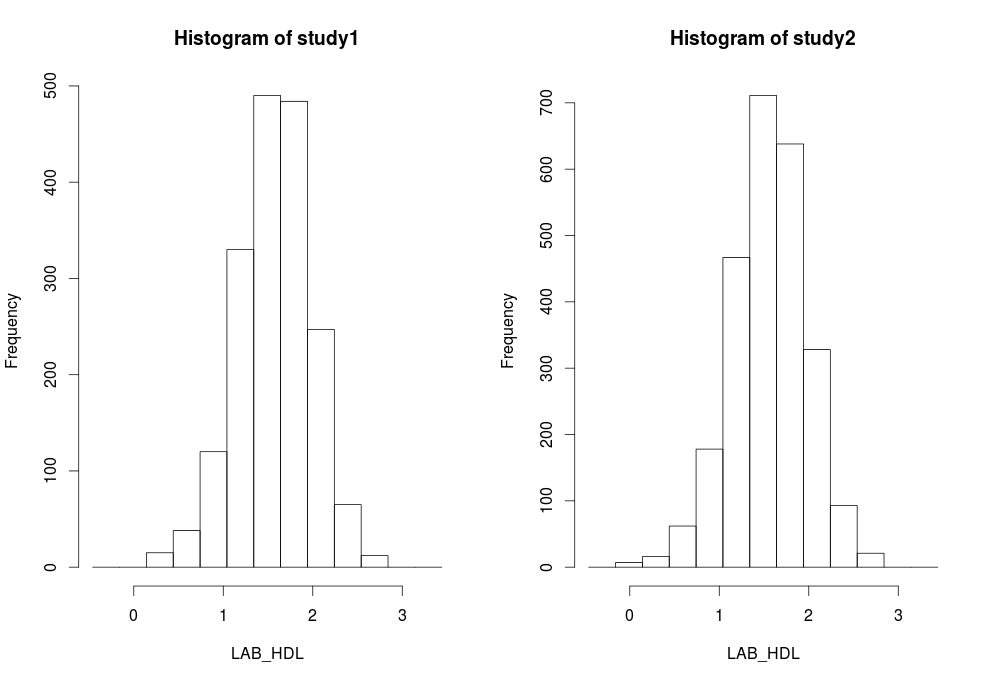
Histograms
| Anchor | ||||
|---|---|---|---|---|
|
| Info | ||
|---|---|---|
| ||
In DataSHIELD histogram outliers are not shown as these are potentially disclosive. The text summary of the function printed to the client screen informs the user of the presence of classes (bins) with a count smaller than the minimal cell count set by data providers. |
...
| Code Block | ||
|---|---|---|
| ||
ds.histogram(x='D$LAB_HDL', type='split') #Warning: study1: 1 invalid cells #Warning: study2: 1 invalid cells |
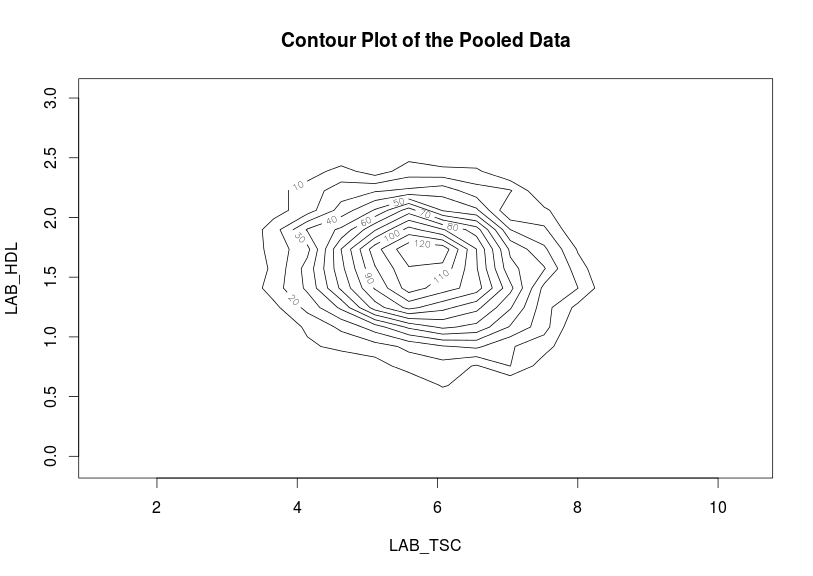
Contour plots
| Anchor | ||||
|---|---|---|---|---|
|
Contour plots are used to visualize a correlation pattern that would traditionally be determined using a scatter plot (which can not be used in DataSHIELD as it is potentially disclosive).
...
| Code Block | ||
|---|---|---|
| ||
ds.contourPlot(x='D$LAB_TSC', y='D$LAB_HDL') #study1: Number of invalid cells (cells with counts >0 and <5) is 83 #study2: Number of invalid cells (cells with counts >0 and <5) is 97 |
Heat map plots
| Anchor | ||||
|---|---|---|---|---|
|
An alternative way to visualise correlation between variables is via a heat map plot.
...
| Note |
|---|
The functions ds.contourPlot and ds.heatmapPlot use the range (mimumum and maximum values) of the x and y vectors in the process of generating the graph. But in DataSHIELD the minimum and maximum values cannot be returned because they are potentially disclosive; hence what is actually returned for these plots is the 'obscured' minimum and maximum. As a consequence the number of invalid cells, in the grid density matrix used for the plot, reported after running the functions can change slightly from one run to another. In the above output for example the number of invalid cells are respectively 83 and 97 for study1 and study2. These figures can change if the command is ran again but we should not be alarmed by this as it does not affect the plot itself. It was a deliberate decision to ensure the real minimum and maximum values are not returned. |
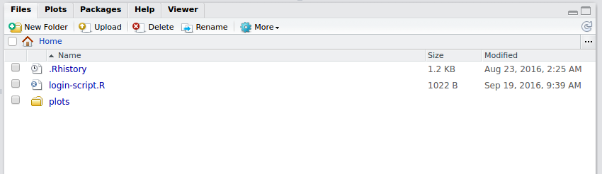
Saving Graphs / Plots in R Studio
- Any plots will appear in the bottom right window in R Studio, within the
plottab - Select
export>save as image
...
- The plot will now be accessible from your Home folder directory structure. On a live DataSHIELD system you can then transfer the plot to your computer via secure file transfer (sftp).
Sub-setting
| Info | ||
|---|---|---|
| ||
Sub-setting is particularly useful in statistical analyses to break down variables or tables of variables into groups for analysis. Repeated sub-setting, however, can lead to thinning of the data to individual-level records that are disclosive (e.g. the statistical mean of a single value point is the value itself). Therefore, DataSHIELD does not subset an object below the minimal cell count set by the data providers (typically this is ≤ 4 observations). |
...
| Anchor | ||||
|---|---|---|---|---|
|
Sub-setting using ds.subsetByClass
- The
ds.subsetByClassfunction generates subsets for each level of acategoricalvariable. If the input is a data frame it produces a subset of that data frame for each class of each categorical variable held in the data frame. - Best practice is to state the categorical variable(s) to subset using the
variablesargument, and the name of the subset data using thesubsetsargument. - The example subsets
GENDERfrom our assigned data frameD, the subset data is namedGenderTables:
...
| Note |
|---|
Running ds.subsetByClass on a data frame without specifying the categorical variable in the argument |
| Anchor | ||||
|---|---|---|---|---|
|
Sub-setting using ds.names
In the previous example, the GENDER variable in assigned data frame D had females coded as 0 and males coded as 1. When GENDER was subset using the ds.subsetByClass function, two subset tables were generated for each study dataset
one for females and one for males.
...
| Anchor | ||||
|---|---|---|---|---|
|
Sub-setting using ds.meanByClass
The ds.meanByClass function generates subset tables similar to ds.subsetByClass but additionally calculates the mean, standard deviation and size for each subset for specific numeric variables.
...
| Note |
|---|
The |
| Anchor | ||||
|---|---|---|---|---|
|
Sub-setting using ds.subset
The function ds.subset allows general sub-setting of different data types e.g. categorical, numeric, character, data frame, matrix. It is also possible to subset rows (the individual records). No output is returned to the client screen, the generated subsets are stored in the server-side R session.
...
| Code Block | ||
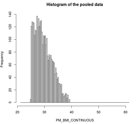
|---|---|---|
| ||
ds.histogram('BMI25plus$PM_BMI_CONTINUOUS') |
Modelling
Horizontal DataSHIELD allows the fitting of:
...
In GLM function the outcome can be modelled as continuous, or categorical (binomial or discrete). The error to use in the model can follow a range of distribution including gaussian, binomial, Gamma and poisson. In this section only one example will be shown, for more examples please see the manual help page for the function.
| Anchor | ||||
|---|---|---|---|---|
|
Generalised linear models
The function
ds.glmis used to analyse the outcome variableDIS_DIAB(diabetes status) and the covariatesPM_BMI_CONTINUOUS(continuous BMI),LAB_HDL(HDL cholesterol) andGENDER(gender), with an interaction between the latter two. In R this model is represented asCode Block D$DIS_DIAB ~ D$PM_BMI_CONTINUOUS+D$LAB_HDL*D$GENDER
By default intermediate results are not printed to the client screen. It is possible to display the intermediate results, to show the coefficients after each iteration, by using the argument
display=TRUE.
...