...

Note

title	Prerequisites

It is recommended that you familiarise yourself with R first by sitting our Introduction to R tutorial.

It also requires that you have the DataSHIELD training environment installed on your machine, see our Installation Instructions for Linux, Windows, or Mac.

Tip

title	Help

DataSHIELD support is freely available in the DataSHIELD forum by the DataSHIELD community. Please use this as the first port of call for any problems you may be having, it is monitored closely for new threads.

DataSHIELD bespoke user support and also user training classes are offered on a fee-paying basis. Please enquire at datashield@newcastle.ac.uk for current prices.

...

This is the fourth in a 6-part DataSHIELD tutorial series. Please see below for links to all prior and subsequent parts:

...

The other parts in this DataSHIELD tutorial series are:

1: Introduction and logging in
Basic 2: Basic statistics and data manipulations
3: Assign functions and tables
Plotting 4: Plotting graphs
Subsetting
5: Subsetting
6: Modelling

Quick reminder for logging in:

Expand

Follow instructions to Start the Opal VMs.

Recall from the installation instructions, the Opal web interface is a simple check to tell if the VMs have started. Load the following urls, waiting at least 1 minute after starting the training VMs.

Start R/RStudio

Load Packages

code login dataframe

Start R/RStudio

Load Packages

Code Block

	xml
	xml

#load libraries
library(DSI)
library(DSOpal)
library(dsBaseClient)

Build your login dataframe

Code Block

language	xml
title	Build your

builder <- DSI::newDSLoginBuilder() builder$append(server = "study1", url = "http://192.168.56.100:8080/", user = "administrator", password = "datashield_test&", table = "CNSIM.CNSIM1

login dataframe

builder <- DSI::newDSLoginBuilder()
builder <- DSI::newDSLoginBuilder()
builder$append(server = "server1", url = "https://opal-demo.obiba.org/",
user = "dsuser", password = "P@ssw0rd", driver = "OpalDriver", options='list(ssl_verifyhost=0, ssl_verifypeer=0)')
builder$append(server = "

study2

server2", url = "

http

https://

192

opal-demo.

168.56.101:8080/",

obiba.org/",
user = "

administrator

dsuser", password = "

datashield_test&

P@ssw0rd",

table

driver = "

CNSIM.CNSIM2

OpalDriver",

driver = "OpalDriver"

options='list(ssl_verifyhost=0, ssl_verifypeer=0)')

logindata <- builder$build()

logindata <- builder$build()

connections <- DSI::datashield.login(logins = logindata, assign = TRUE)
DSI::datashield.assign.table(conns = connections, symbol =

"D"

"DST", table = c("CNSIM.CNSIM1","CNSIM.CNSIM2"))

Command to logout:

Code Block

language	bash

DSI::datashield.logout(connections)

Generating graphs

It is currently possible to produce 4 types of graphs in DataSHIELD: histograms, contour plots, heatmap plots and scatter plots.

...

The ds.histogram function can be used to create a histogram of LAB_HDL that is in the assigned variable dataframe (named "DDST", by default). The default analysis is set to run on separate data from all studies. Note that Study 1 contains 2 invalid cells (bins) - those bins contain counts less than the data provider minimal cell count.

...

Code Block

language	xml

ds.histogram(x='D$LABDST$LAB_HDL', datasources = connections)

...

Code Block

language	xml
theme	RDark

  Aggregated (exists("DDST")) [=============================================================] 100% / 0s
  Aggregated (classDS("D$LABDST$LAB_HDL")) [====================================================] 100% / 0s
  Aggregated (histogramDS1(D$LABDST$LAB_HDL,1,3,0.25)) [========================================] 100% / 0s
  Aggregated (histogramDS2(D$LABDST$LAB_HDL,10,-0.153421749557465,3.0579610811785,1,3,0.25)) [==] 100% / 0s
Warning: study1: 2 invalid cells
Warning: study2: 0 invalid cells
[[1]]
$breaks
 [1] -0.1534217  0.1677165  0.4888548  0.8099931  1.1311314  1.4522697  1.7734079  2.0945462  2.4156845  2.7368228
[11]  3.0579611

$counts
 [1]   0  18  51 172 443 550 387 153  25   0

$density
 [1] 0.00000000 0.03108742 0.08808103 0.29705758 0.76509598 0.94989343 0.66837956 0.26424308 0.04317697 0.00000000

$mids
 [1] 0.007147392 0.328285675 0.649423958 0.970562241 1.291700524 1.612838807 1.933977090 2.255115373 2.576253657
[10] 2.897391940

$xname
[1] "xvect"

$equidist
[1] TRUE

attr(,"class")
[1] "histogram"

[[2]]
$breaks
 [1] -0.1534217  0.1677165  0.4888548  0.8099931  1.1311314  1.4522697  1.7734079  2.0945462  2.4156845  2.7368228
[11]  3.0579611

$counts
 [1]   9  19  83 275 604 769 545 182  42   5

$density
 [1] 0.01106408 0.02335750 0.10203539 0.33806906 0.74252258 0.94536402 0.66999140 0.22374025 0.05163237 0.00614671

$mids
 [1] 0.007147392 0.328285675 0.649423958 0.970562241 1.291700524 1.612838807 1.933977090 2.255115373 2.576253657
[10] 2.897391940

$xname
[1] "xvect"

$equidist
[1] TRUE

attr(,"class")
[1] "histogram"

...

Code Block

language	xml

ds.histogram(x='D$LABDST$LAB_HDL', type = 'combine', datasources = connections)

...

Code Block

language	xml
theme	RDark

  Aggregated (exists("DDST")) [=============================================================] 100% / 0s
  Aggregated (classDS("D$LABDST$LAB_HDL")) [====================================================] 100% / 0s
  Aggregated (histogramDS1(D$LABDST$LAB_HDL,1,3,0.25)) [========================================] 100% / 0s
  Aggregated (histogramDS2(D$LABDST$LAB_HDL,10,-0.153421749557465,3.0579610811785,1,3,0.25)) [==] 100% / 0s
$breaks
 [1] -0.1534217  0.1677165  0.4888548  0.8099931  1.1311314  1.4522697  1.7734079  2.0945462  2.4156845  2.7368228
[11]  3.0579611

$counts
 [1]    9   37  134  447 1047 1319  932  335   67    5

$density
 [1] 0.003688026 0.018148307 0.063372138 0.211708879 0.502539521 0.631752481 0.446123653 0.162661110 0.031603113
[10] 0.002048903

$mids
 [1] 0.007147392 0.328285675 0.649423958 0.970562241 1.291700524 1.612838807 1.933977090 2.255115373 2.576253657
[10] 2.897391940

$xname
[1] "xvect"

$equidist
[1] TRUE

$intensities
 [1] 0.003688026 0.018148307 0.063372138 0.211708879 0.502539521 0.631752481 0.446123653 0.162661110 0.031603113
[10] 0.002048903

attr(,"class")
[1] "histogram"

...

Code Block

language	xml

ds.contourPlot(x='D$LABDST$LAB_TSC', y='D$LABDST$LAB_HDL', datasources = connections)

...

Code Block

language	xml

ds.heatmapPlot(x='D$LABDST$LAB_TSC', y='D$LABDST$LAB_HDL', datasources = connections)

...

Code Block

language	xml
theme	RDark

  Aggregated (exists("DDST")) [=============================================================] 100% / 0s
  Aggregated (exists("DDST")) [=============================================================] 100% / 0s
  Aggregated (classDS("D$LABDST$LAB_TSC")) [====================================================] 100% / 0s
  Aggregated (classDS("D$LABDST$LAB_HDL")) [====================================================] 100% / 0s
  Aggregated (rangeDS( D$LABDST$LAB_TSC )) [====================================================] 100% / 0s
  Aggregated (rangeDS( D$LABDST$LAB_HDL )) [====================================================] 100% / 0s
  Aggregated (densityGridDS(D$LABDST$LAB_TSC,D$LABDST$LAB_HDL,TRUE,1.03336178741064,10.5673103958328,-0.1460271...
study1: Number of invalid cells (cells with counts >0 and < nfilter.tab ) is 63
study2: Number of invalid cells (cells with counts >0 and < nfilter.tab ) is 74

...

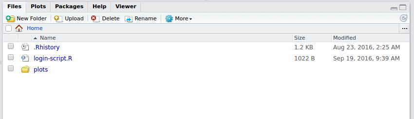
The plot will now be accessible from your Home folder directory structure.

Conclusion

The next part other parts in this DataSHIELD tutorial series isare:

...

1: Introduction and logging in

...

Plotting graphs

...

Subsetting <-

Tip

Also remember you can:

get a function list for any DataSHIELD package and
view the manual help page individual functions
in the DataSHIELD test environment it is possible to print analyses to file (.csv, .txt, .pdf, .png)
take a look at our FAQ page for solutions to common problems such as Changing variable class to use in a specific DataSHIELD function.
Get support from our DataSHIELD forum.

...

Versions Compared

Old Version 2

New Version Current

Key

Quick reminder for logging in:

Start R/RStudio

Load Packages

Start R/RStudio

Load Packages

Build your login dataframe

Generating graphs

Conclusion

Page Comparison

Versions Compared

Old Version 2

New Version Current

Key

Quick reminder for logging in:

Start R/RStudio

Load Packages

Start R/RStudio

Load Packages

Build your login dataframe

Generating graphs

Conclusion