DataSHIELD Training Part 4: Plotting graphs
- Alex Westerberg (Unlicensed)
- Becca Wilson
Prerequisites
It is recommended that you familiarise yourself with R first by sitting our Introduction to R tutorial.
It also requires that you have the DataSHIELD training environment installed on your machine, see our Installation Instructions for Linux, Windows, or Mac.
Help
DataSHIELD support is freely available in the DataSHIELD forum by the DataSHIELD community. Please use this as the first port of call for any problems you may be having, it is monitored closely for new threads.
DataSHIELD bespoke user support and also user training classes are offered on a fee-paying basis. Please enquire at datashield@newcastle.ac.uk for current prices.
Introduction
This is the fourth in a 6-part DataSHIELD tutorial series.
The other parts in this DataSHIELD tutorial series are:
5: Subsetting
6: Modelling
Quick reminder for logging in:
Generating graphs
It is currently possible to produce 4 types of graphs in DataSHIELD: histograms, contour plots, heatmap plots and scatter plots.
Histograms
Histograms
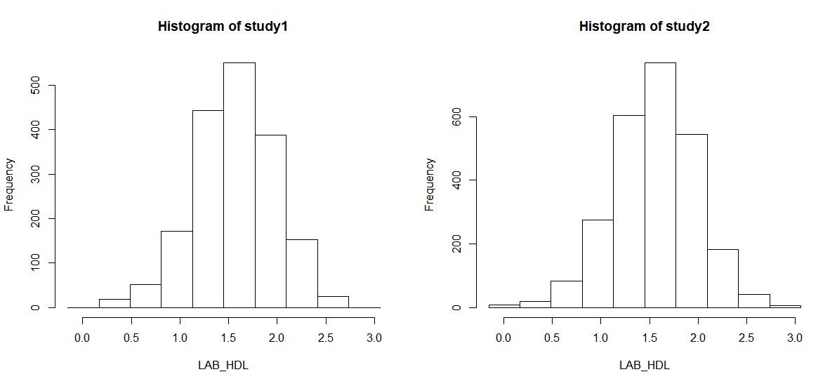
In the default method of generating a DataSHIELD histogram outliers are not shown as these are potentially disclosive. The text summary of the function printed to the client screen informs the user of the presence of classes (bins) with a count smaller than the minimal cell count set by data providers.
Note that a small random number is added to the minimum and maximum values of the range of the input variable. Therefore each user should expect slightly different printed results from those shown below:
- The
ds.histogramfunction can be used to create a histogram ofLAB_HDLthat is in the assigned variable dataframe (named "DST", by default). The default analysis is set to run on separate data from all studies. Note that Study 1 contains 2 invalid cells (bins) - those bins contain counts less than the data provider minimal cell count.
ds.histogram(x='DST$LAB_HDL', datasources = connections)
  Aggregated (exists("DST")) [=============================================================] 100% / 0s
  Aggregated (classDS("DST$LAB_HDL")) [====================================================] 100% / 0s
  Aggregated (histogramDS1(DST$LAB_HDL,1,3,0.25)) [========================================] 100% / 0s
  Aggregated (histogramDS2(DST$LAB_HDL,10,-0.153421749557465,3.0579610811785,1,3,0.25)) [==] 100% / 0s
Warning: study1: 2 invalid cells
Warning: study2: 0 invalid cells
[[1]]
$breaks
 [1] -0.1534217  0.1677165  0.4888548  0.8099931  1.1311314  1.4522697  1.7734079  2.0945462  2.4156845  2.7368228
[11]  3.0579611

$counts
 [1]   0  18  51 172 443 550 387 153  25   0

$density
 [1] 0.00000000 0.03108742 0.08808103 0.29705758 0.76509598 0.94989343 0.66837956 0.26424308 0.04317697 0.00000000

$mids
 [1] 0.007147392 0.328285675 0.649423958 0.970562241 1.291700524 1.612838807 1.933977090 2.255115373 2.576253657
[10] 2.897391940

$xname
[1] "xvect"

$equidist
[1] TRUE

attr(,"class")
[1] "histogram"

[[2]]
$breaks
 [1] -0.1534217  0.1677165  0.4888548  0.8099931  1.1311314  1.4522697  1.7734079  2.0945462  2.4156845  2.7368228
[11]  3.0579611

$counts
 [1]   9  19  83 275 604 769 545 182  42   5

$density
 [1] 0.01106408 0.02335750 0.10203539 0.33806906 0.74252258 0.94536402 0.66999140 0.22374025 0.05163237 0.00614671

$mids
 [1] 0.007147392 0.328285675 0.649423958 0.970562241 1.291700524 1.612838807 1.933977090 2.255115373 2.576253657
[10] 2.897391940

$xname
[1] "xvect"

$equidist
[1] TRUE

attr(,"class")
[1] "histogram"
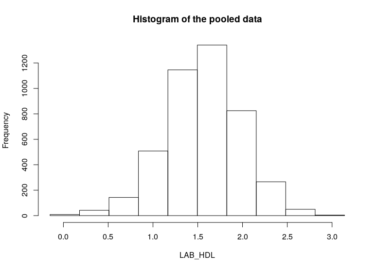
- To produce histograms from a pooled study, the argument
type='combine'is used.
ds.histogram(x='DST$LAB_HDL', type = 'combine', datasources = connections)
  Aggregated (exists("DST")) [=============================================================] 100% / 0s
  Aggregated (classDS("DST$LAB_HDL")) [====================================================] 100% / 0s
  Aggregated (histogramDS1(DST$LAB_HDL,1,3,0.25)) [========================================] 100% / 0s
  Aggregated (histogramDS2(DST$LAB_HDL,10,-0.153421749557465,3.0579610811785,1,3,0.25)) [==] 100% / 0s
$breaks
 [1] -0.1534217  0.1677165  0.4888548  0.8099931  1.1311314  1.4522697  1.7734079  2.0945462  2.4156845  2.7368228
[11]  3.0579611

$counts
 [1]    9   37  134  447 1047 1319  932  335   67    5

$density
 [1] 0.003688026 0.018148307 0.063372138 0.211708879 0.502539521 0.631752481 0.446123653 0.162661110 0.031603113
[10] 0.002048903

$mids
 [1] 0.007147392 0.328285675 0.649423958 0.970562241 1.291700524 1.612838807 1.933977090 2.255115373 2.576253657
[10] 2.897391940

$xname
[1] "xvect"

$equidist
[1] TRUE

$intensities
 [1] 0.003688026 0.018148307 0.063372138 0.211708879 0.502539521 0.631752481 0.446123653 0.162661110 0.031603113
[10] 0.002048903

attr(,"class")
[1] "histogram"
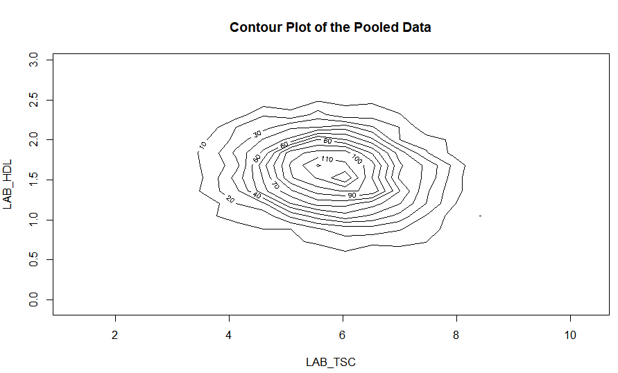
Contour plots
Contour plots are used to visualize a correlation pattern.
- The function
ds.contourPlotis used to visualise the correlation between the variablesLAB_TSC(total serum cholesterol andLAB_HDL(HDL cholesterol). The default istype='combined'- the results represent a contour plot on pooled data across all studies:
ds.contourPlot(x='DST$LAB_TSC', y='DST$LAB_HDL', datasources = connections)
  Aggregated (exists("D")) [=============================================================] 100% / 0s
  Aggregated (exists("D")) [=============================================================] 100% / 0s
  Aggregated (classDS("D$LAB_TSC")) [====================================================] 100% / 0s
  Aggregated (classDS("D$LAB_HDL")) [====================================================] 100% / 0s
  Aggregated (rangeDS(D$LAB_TSC)) [======================================================] 100% / 0s
  Aggregated (rangeDS(D$LAB_HDL)) [======================================================] 100% / 0s
  Aggregated (densityGridDS(D$LAB_TSC,D$LAB_HDL,TRUE,1.03336178741064,10.5673103958328,-0.1460271...
study1: Number of invalid cells (cells with counts >0 and < nfilter.tab ) is 63
study2: Number of invalid cells (cells with counts >0 and < nfilter.tab ) is 74
Heat map plots
An alternative way to visualise correlation between variables is via a heat map plot.
- The function
ds.heatmapPlotis applied to the variablesLAB_TSCandLAB_HDL:
ds.heatmapPlot(x='DST$LAB_TSC', y='DST$LAB_HDL', datasources = connections)
  Aggregated (exists("DST")) [=============================================================] 100% / 0s
  Aggregated (exists("DST")) [=============================================================] 100% / 0s
  Aggregated (classDS("DST$LAB_TSC")) [====================================================] 100% / 0s
  Aggregated (classDS("DST$LAB_HDL")) [====================================================] 100% / 0s
  Aggregated (rangeDS( DST$LAB_TSC )) [====================================================] 100% / 0s
  Aggregated (rangeDS( DST$LAB_HDL )) [====================================================] 100% / 0s
  Aggregated (densityGridDS(DST$LAB_TSC,DST$LAB_HDL,TRUE,1.03336178741064,10.5673103958328,-0.1460271...
study1: Number of invalid cells (cells with counts >0 and < nfilter.tab ) is 63
study2: Number of invalid cells (cells with counts >0 and < nfilter.tab ) is 74
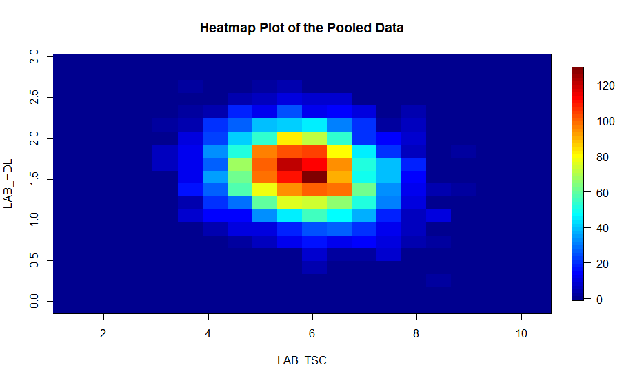
The functions ds.contourPlot and ds.heatmapPlot use the range (minimum and maximum values) of the x and y vectors in the process of generating the graph. But in DataSHIELD the minimum and maximum values cannot be returned because they are potentially disclosive; hence what is actually returned for these plots is the 'obscured' minimum and maximum.
Saving Graphs / Plots in R Studio
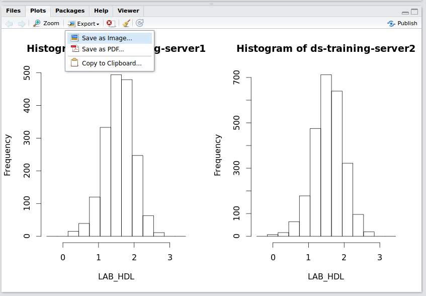
- Any plots will appear in the bottom right window in R Studio, within the
plottab - Select
export>save as image
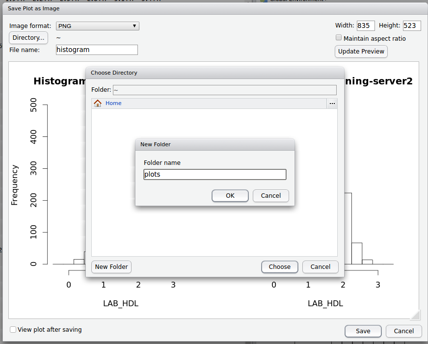
- Name the file and select / create a folder to store the image in on the DataSHIELD Client server.
- You can also edit the width and height of the graph
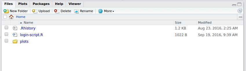
- The plot will now be accessible from your Home folder directory structure.
Conclusion
The other parts in this DataSHIELD tutorial series are:
- 1: Introduction and logging in
- 2: Basic statistics and data manipulations
- 3: Assign functions and tables
- 4: Plotting graphs
- 5: Subsetting
- 6: Modelling
Also remember you can:
- get a function list for any DataSHIELD package and
- view the manual help page individual functions
- in the DataSHIELD test environment it is possible to print analyses to file (.csv, .txt, .pdf, .png)
- take a look at our FAQ page for solutions to common problems such as Changing variable class to use in a specific DataSHIELD function.
- Get support from our DataSHIELD forum.

DataSHIELD Wiki by DataSHIELD is licensed under a Creative Commons Attribution-ShareAlike 4.0 International License. Based on a work at http://www.datashield.ac.uk/wiki