Session 3: DataSHIELD extended practical session answers
- Former user (Deleted)
- Becca Wilson
- Former user (Deleted)
# load libraries
library(opal)
library(dsBaseClient)
library(dsStatsClient)
library(dsGraphicsClient)
library(dsModellingClient)

server <- c("study1", "study2", "study3")
url <- c("http://XXXXXX:8080")
table <- c("DASIM.DASIM1", "DASIM.DASIM2", "DASIM.DASIM3")
logindata <- data.frame(server,url,user="administrator",password="datashield_test&",table)

# login and assign the whole dataset
opals <- datashield.login(logins=logindata,assign=TRUE)
Subsets and Statistics
- Calculate the mean and the variance of the continuous variable BMI of obese males.
# Check the levels of categorigal BMI (1=normal, 2=overweight, 3=obese)
ds.levels('D$PM_BMI_CATEGORICAL')

# Check the levels of gender (0=males, 1=females)
ds.levels('D$GENDER')

# Create a subset dataset that includes only the obese people
ds.subset(x='D', subset='BMI_3', logicalOperator='PM_BMI_CATEGORICAL==', threshold=3)

# See how many obese people are in each study
ds.dim('BMI_3')

# Create a subset dataset that includes only the obese males
ds.subset(x='BMI_3', subset='BMI_3_males', logicalOperator='GENDER==', threshold=0)

# Check how many obese males are in each study
ds.dim('BMI_3_males')

# Calculate the global mean and global variance of continuous bmi for obese males
ds.mean('BMI_3_males$PM_BMI_CONTINUOUS')
ds.var('BMI_3_males$PM_BMI_CONTINUOUS')
Answer: Question 1
The global mean and the global variance of BMI are 33.04723 and 6.134642 respectively.Assign and Plots
Find the quantile mean and plot a histogram of pooled data for the exponent and for the logarithm of LAB_HDL measurement.
# Assign a new variable which gives the exponents of HDL
ds.exp(x='D$LAB_HDL', newobj='exp_hdl')

# Find the quantile mean of the exponents of HDL
ds.quantileMean('exp_hdl')

# Plot a histogram for the exponents of HDL
ds.histogram('exp_hdl')
Answer: Question 2
Quantiles of the pooled data 5% 10% 25% 50% 75% 90% 95% Mean
2.555388 2.922673 3.660593 4.727446 6.072125 7.653894 8.725955 5.066809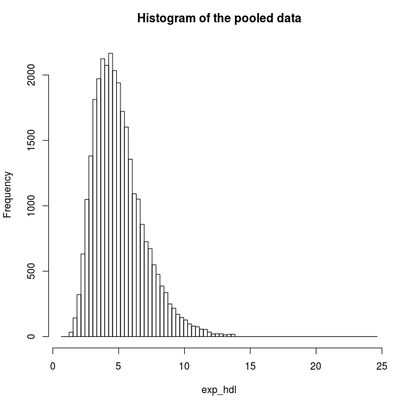
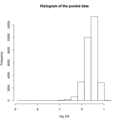
# Assign a new variable which gives the logarithms of HDL
ds.log(x='D$LAB_HDL', newobj='log_hdl')

# Find the quantile mean of the logarithms of HDL
ds.quantileMean('log_hdl')

# Plot a histogram for the logarithms of HDL
ds.histogram('log_hdl')
Answer: Question 2 continued
Quantiles of the pooled data
5% 10% 25% 50% 75% 90%
-0.06384112 0.06994799 0.26052368 0.44043450 0.58983773 0.71059831
95% Mean
0.77301979 0.40754040
2-dimensional contingency tables
- What percentage of females (pooled data) are diabetics?
- What percentage of males in each study separately have stroke (DIS_CVA)?
# Produce a two dimensional table for the variables GENDER and DIS_DIAB for combined data
ds.table2D(x='D$GENDER', y='D$DIS_DIAB')
Answer: Question 3
1.57% of females (pooled data) are diabetics.$counts $counts$`pooled-D$GENDER(row)|D$DIS_DIAB(col)` 0 1 Total 0 14830 158 14988 1 14777 235 15012 Total 29607 393 30000 $rowPercent $rowPercent$`pooled-D$GENDER(row)|D$DIS_DIAB(col)` 0 1 Total 0 98.95 1.05 100 1 98.43 1.57 100 Total 98.69 1.31 100 $colPercent $colPercent$`pooled-D$GENDER(row)|D$DIS_DIAB(col)` 0 1 Total 0 50.09 40.2 49.96 1 49.91 59.8 50.04 Total 100.00 100.0 100.00 $chi2Test $chi2Test$`pooled-D$GENDER(row)|D$DIS_DIAB(col)` Pearson's Chi-squared test with Yates' continuity correction data: pooledContingencyTable X-squared = 14.769, df = 1, p-value = 0.0001215 $validity [1] "All tables are valid!"
# Produce a two dimensional table for the variables GENDER and DIS_CVA for split data
ds.table2D(x='D$GENDER',y='D$DIS_CVA', type='split')
Answer: Question 3 continued
The percentages of males having stroke are 0.82% in study 1, 0.80% in study 2 and 0.78% in study 3.$counts
$counts$`study1-D$GENDER(row)|D$DIS_CVA(col)`
0 1 Total
0 4955 41 4996
1 4979 25 5004
Total 9934 66 10000
$counts$`study2-D$GENDER(row)|D$DIS_CVA(col)`
0 1 Total
0 4956 40 4996
1 4970 34 5004
Total 9926 74 10000
$counts$`study3-D$GENDER(row)|D$DIS_CVA(col)`
0 1 Total
0 4960 36 4996
1 4976 28 5004
Total 9936 64 10000
$rowPercent
$rowPercent$`study1-D$GENDER(row)|D$DIS_CVA(col)`
0 1 Total
0 99.18 0.82 100
1 99.50 0.50 100
Total 99.34 0.66 100
$rowPercent$`study2-D$GENDER(row)|D$DIS_CVA(col)`
0 1 Total
0 99.20 0.80 100
1 99.32 0.68 100
Total 99.26 0.74 100
$rowPercent$`study3-D$GENDER(row)|D$DIS_CVA(col)`
0 1 Total
0 99.28 0.72 100
1 99.44 0.56 100
Total 99.36 0.64 100
$colPercent
$colPercent$`study1-D$GENDER(row)|D$DIS_CVA(col)`
0 1 Total
0 49.88 62.12 49.96
1 50.12 37.88 50.04
Total 100.00 100.00 100.00
$colPercent$`study2-D$GENDER(row)|D$DIS_CVA(col)`
0 1 Total
0 49.93 54.05 49.96
1 50.07 45.95 50.04
Total 100.00 100.00 100.00
$colPercent$`study3-D$GENDER(row)|D$DIS_CVA(col)`
0 1 Total
0 49.92 56.25 49.96
1 50.08 43.75 50.04
Total 100.00 100.00 100.00
$chi2Test
$chi2Test$`study1-D$GENDER(row)|D$DIS_CVA(col)`
Pearson's Chi-squared test with Yates' continuity correction
data: contingencyTable
X-squared = 3.4559, df = 1, p-value = 0.06302
$chi2Test$`study2-D$GENDER(row)|D$DIS_CVA(col)`
Pearson's Chi-squared test with Yates' continuity correction
data: contingencyTable
X-squared = 0.34846, df = 1, p-value = 0.555
$chi2Test$`study3-D$GENDER(row)|D$DIS_CVA(col)`
Pearson's Chi-squared test with Yates' continuity correction
Generalized Linear Models
- Apply a generalised linear model that predicts the level of glucose between males and females. What is the predicted average level of glucose for males? What is this value for females?
- Apply a GLM to predict the level of glucose using gender and continuous bmi. How much the level of glucose is increasing with the increase of bmi by one unit? What is the predicted glucose level of a female with bmi=22?
# Apply GLM to find the linear relatioship between LAB_GLUC_FASTING and GENDER
ds.glm("D$LAB_GLUC_FASTING ~ 1 + D$GENDER",family="gaussian")
Answer: Question 4
The relationship between glucose and gender is given by the formula:
LAB_GLUC_FASTING=4.62223776-0.08929719*GENDER
For males, GENDER=0 and therefore their average level of glucose
is 4.62223776
For females, GENDER=1 and therefore their average level of glucoseis 4.62223776-0.08929719=4.532941.
$formula
[1] "D$LAB_GLUC_FASTING ~ 1 + D$GENDER"


$family
Family: gaussian
Link function: identity


$coefficients
                             Estimate        Std. Error        z-value              p-value       low0.95CI
(Intercept)     4.62223776  0.005806318  796.07035  0.000000e+00     4.6108576
GENDER1     -0.08929719  0.008208091 -10.87917   1.448816e-27     -0.1053848
                       high0.95CI
(Intercept)    4.63361793
GENDER1     -0.07320963


$dev
[1] 15157.85


$df
[1] 29998


$nsubs
[1] 30000


$iter
[1] 3


attr(,"class")
[1] "glmds"
# Apply GLM to find the linear relatioship of LAB_GLUC_FASTING with GENDER and PM_BMI_CONTINUOUS
ds.glm("D$LAB_GLUC_FASTING~1+D$GENDER+D$PM_BMI_CONTINUOUS",family="gaussian")
Answer: Question 4 continued
The level of glucose related to gender and bmi is given by the formula:
LAB_GLUC_FASTING=3.64750965-0.07493214*GENDER+0.03543909*PM_BMI_CONTINUOUS
While the level of bmi is increasing by one unit, the level of glucose is
increasing by 0.03543909.
For a female (GENDER=1) with PM_BMI_CONTINUOUS=22, the level of glucose
should be 3.64750965-0.07493214*1+0.03543909*22=4.352237
 $formula
[1] "D$LAB_GLUC_FASTING ~ 1 + D$GENDER + D$PM_BMI_CONTINUOUS"


$family
Family: gaussian
Link function: identity


$coefficients
                                 Estimate           Std. Error          z-value              p-value     low0.95CI
(Intercept)        3.64750965   0.0237582722  153.525880 0.000000e+00  3.60094429
GENDER1           -0.07493214 0.0079817991  -9.387876    6.122208e-21  -0.09057618
PM_BMI_CONTINUOUS  0.03543909 0.0008390991  42.234690 0.000000e+00  0.03379449
                            high0.95CI
(Intercept)        3.6940750
GENDER1          -0.0592881
PM_BMI_CONTINUOUS  0.0370837


$dev
[1] 14307.08


$df
[1] 29997


$nsubs
[1] 30000


$iter
[1] 3


attr(,"class")
[1] "glmds"
# clear the Datashield R sessions and logout
datashield.logout(opals)
Related content

DataSHIELD Wiki by DataSHIELD is licensed under a Creative Commons Attribution-ShareAlike 4.0 International License. Based on a work at http://www.datashield.ac.uk/wiki