Click here for page contents...

Prerequisites

It is recommended that you familiarise yourself with R first by sitting our Introduction to R tutorial.

It also requires that you have the DataSHIELD training environment installed on your machine, see our Installation Instructions for Linux, Windows, or Mac.

Help

DataSHIELD support is freely available in the DataSHIELD forum by the DataSHIELD community. Please use this as the first port of call for any problems you may be having, it is monitored closely for new threads.

DataSHIELD bespoke user support and also user training classes are offered on a fee-paying basis. Please enquire at datashield@newcastle.ac.uk for current prices.

Introduction

This is the fifth in a 6-part DataSHIELD tutorial series.

The other parts in this DataSHIELD tutorial series are:

1: Introduction and logging in
2: Basic statistics and data manipulations
3: Assign functions and tables
4: Plotting graphs
5: Sub-setting
6: Modelling

Quick reminder for logging in:

Click here to expand...

Follow instructions to Start the Opal VMs.

Recall from the installation instructions, the Opal web interface is a simple check to tell if the VMs have started. Load the following urls, waiting at least 1 minute after starting the training VMs.

Start R/RStudio

Load Packages

#load libraries
library(DSI)
library(DSOpal)
library(dsBaseClient)

Build your login dataframe

Build your login dataframe

builder <- DSI::newDSLoginBuilder()
builder$append(server = "study1",  url = "http://192.168.56.100:8080/",
               user = "administrator", password = "datashield_test&",
               table = "CNSIM.CNSIM1", driver = "OpalDriver")
builder$append(server = "study2", url = "http://192.168.56.101:8080/",
               user = "administrator", password = "datashield_test&",
               table = "CNSIM.CNSIM2", driver = "OpalDriver")

logindata <- builder$build()

connections <- DSI::datashield.login(logins = logindata, assign = TRUE, symbol = "D")

Command to logout:

DSI::datashield.logout(connections)

Sub-setting

Limitations on subsetting

Sub-setting is particularly useful in statistical analyses to break down variables or tables of variables into groups for analysis. Repeated sub-setting, however, can lead to thinning of the data to individual-level records that are disclosive (e.g. the statistical mean of a single value point is the value itself). Therefore, DataSHIELD does not subset an object below the minimal subset length set by the data providers (typically this is ≤ 4 observations).

In DataSHIELD there is one function that allows sub-setting of data, ds.dataFrameSubset .

You may wish to use it to:

Subset a column of data by its "Class"
Subset a dataframe to remove any "NA"s
Subset a numeric column of a dataframe using a Boolean inequalilty

Sub-setting by class

You may wish to generate subsets for each level of a categorical variable. To do this we must think about which levels of that categorical variable are available, then use boolean operators to isolate them:

# first find the column name you wish to refer to
ds.colnames(x="D")
# then check which levels you need to apply a boolean operator to:
ds.levels(x="D$GENDER")
?ds.dataFrameSubset

At this stage, we want to work out what arguments are available in the DataSHIELD function so we summon the function help; the help appears as:

ds.dataFrameSubset(
  df.name = NULL,
  V1.name = NULL,
  V2.name = NULL,
  Boolean.operator = NULL,
  keep.cols = NULL,
  rm.cols = NULL,
  keep.NAs = NULL,
  newobj = NULL,
  datasources = NULL,
  notify.of.progress = FALSE
)
Arguments
df.name	
a character string providing the name of the data frame to be subseted.

V1.name	
A character string specifying the name of the vector to which the Boolean operator is to be applied to define the subset. For more information see details.

V2.name	
A character string specifying the name of the vector to compare with V1.name.

Boolean.operator	
A character string specifying one of six possible Boolean operators: '==', '!=', '>', '>=', '<' and '<='.

keep.cols	
a numeric vector specifying the numbers of the columns to be kept in the final subset.

rm.cols	
a numeric vector specifying the numbers of the columns to be removed from the final subset.

keep.NAs	
logical, if TRUE the missing values are included in the subset. If FALSE or NULL all rows with at least one missing values are removed from the subset.

newobj	
a character string that provides the name for the output object that is stored on the data servers. Default dataframesubset.newobj.

datasources	
a list of DSConnection-class objects obtained after login. If the datasources the default set of connections will be used: see datashield.connections_default.

notify.of.progress	
specifies if console output should be produced to indicate progress. Default FALSE.

So what we have learnt from this is that we must specify:

the data frame we are working with throughout this tutorial ("D"), as the df.name argument
the column we wish to split by class ("D$GENDER"), as the V1.name argument
the value we want to compare the column with, in this case a number ("0"), as the V2.name argument
the boolean operator we want to use to compare V2.name with V1.name argument
the specific name we want to call the new object, in string form, with the newobj argument
as always, specify the datasources = connections

ds.dataFrameSubset(df.name = "D", V1.name = "D$GENDER", V2.name = "1", Boolean.operator = "==", newobj = "CNSIM.subset.Males", datasources= connections)
ds.dataFrameSubset(df.name = "D", V1.name = "D$GENDER", V2.name = "0", Boolean.operator = "==", newobj = "CNSIM.subset.Females",datasources= connections)

Now there are two serverside objects which have split GENDER by class, to which we have assigned the names "CNSIM.subset.Males" and "CNSIM.subset.Females".

Sub-setting to remove NAs

The example below uses the function ds.completeCases to subset the assigned data frame D by rows (individual records) that have no missing values (missing values are denoted with NA). The output subset is named "D_without_NA":

ds.completeCases(x1="D",newobj="D_without_NA", datasources=connections)

  Assigned expr. (D_without_NA <- completeCasesDS("D")) [================================] 100% / 1s
  Aggregated (testObjExistsDS("D_without_NA")) [=========================================] 100% / 0s
  Aggregated (messageDS("D_without_NA")) [===============================================] 100% / 0s
$is.object.created
[1] "A data object <D_without_NA> has been created in all specified data sources"

$validity.check
[1] "<D_without_NA> appears valid in all sources"

A subsequent check using ds.dim() will confirm that the new object "D_without_NA" has fewer rows than the original object "D".

Sub-set by inequality

Say we wanted to have a subset where BMI values are ≥ 25, and call it subset.BMI.25.plus

Then the V1.name argument should specify the column name for BMI, which is PM_BMI_CONTINUOUS (remember, this can always be checked by the command ds.colnames(x="D") )and the V2.name argument should specify the value to compare the column to, namely 25, using the boolean operator >=. In the DataSHIELD syntax this looks like the following:

ds.dataFrameSubset(df.name = "D",
  V1.name = "D$PM_BMI_CONTINUOUS",
  V2.name = "25",
  Boolean.operator = ">=",
  newobj = "subset.BMI.25.plus",
  datasources = connections)

The output is:

  Aggregated (dataFrameSubsetDS1("D", "D$PM_BMI_CONTINUOUS", "25", 6, NULL, ) [==========] 100% / 1s
  Assigned expr. (subset.BMI.25.plus <- dataFrameSubsetDS2("D", "D$PM_BMI_CONTINUOUS", "25", 6, N...
  Aggregated (testObjExistsDS("subset.BMI.25.plus")) [===================================] 100% / 0s
  Aggregated (messageDS("subset.BMI.25.plus")) [=========================================] 100% / 0s
$is.object.created
[1] "A data object <subset.BMI.25.plus> has been created in all specified data sources"

$validity.check
[1] "<subset.BMI.25.plus> appears valid in all sources"

The subset of data retains the same variables names i.e. column names. Note we are addressing our newly-named object on the serverside, not accessing a column of the original dataframe "D$...." as before:

ds.colnames(x="subset.BMI.25.plus", datasources = connections)

Outputs:

  Aggregated (exists("subset.BMI.25.plus")) [============================================] 100% / 0s
  Aggregated (classDS("subset.BMI.25.plus")) [===========================================] 100% / 0s
  Aggregated (colnamesDS("subset.BMI.25.plus")) [========================================] 100% / 0s
$study1
 [1] "LAB_TSC"            "LAB_TRIG"           "LAB_HDL"            "LAB_GLUC_ADJUSTED"  "PM_BMI_CONTINUOUS" 
 [6] "DIS_CVA"            "MEDI_LPD"           "DIS_DIAB"           "DIS_AMI"            "GENDER"            
[11] "PM_BMI_CATEGORICAL"

$study2
 [1] "LAB_TSC"            "LAB_TRIG"           "LAB_HDL"            "LAB_GLUC_ADJUSTED"  "PM_BMI_CONTINUOUS" 
 [6] "DIS_CVA"            "MEDI_LPD"           "DIS_DIAB"           "DIS_AMI"            "GENDER"            
[11] "PM_BMI_CATEGORICAL"

To verify the subset above is correct (holds only observations with BMI ≥ 25) the function ds.quantileMean with the argument type='split' will confirm the BMI results for each study are ≥ 25.

ds.quantileMean(x="subset.BMI.25.plus$PM_BMI_CONTINUOUS", type = "split", datasources= connections)

Outputs:

  Aggregated (exists("subset.BMI.25.plus")) [============================================] 100% / 0s
  Aggregated (classDS("subset.BMI.25.plus$PM_BMI_CONTINUOUS")) [=========================] 100% / 0s
  Aggregated (quantileMeanDS(subset.BMI.25.plus$PM_BMI_CONTINUOUS)) [====================] 100% / 0s
  Aggregated (lengthDS("subset.BMI.25.plus$PM_BMI_CONTINUOUS")) [========================] 100% / 0s
  Aggregated (numNaDS(subset.BMI.25.plus$PM_BMI_CONTINUOUS)) [===========================] 100% / 0s
$study1
     5%     10%     25%     50%     75%     90%     95%    Mean 
25.3500 25.7100 27.1500 29.2000 32.0600 34.6560 36.4980 29.9019 

$study2
      5%      10%      25%      50%      75%      90%      95%     Mean 
25.46900 25.91800 27.19000 29.27000 32.20500 34.76200 36.24300 29.92606

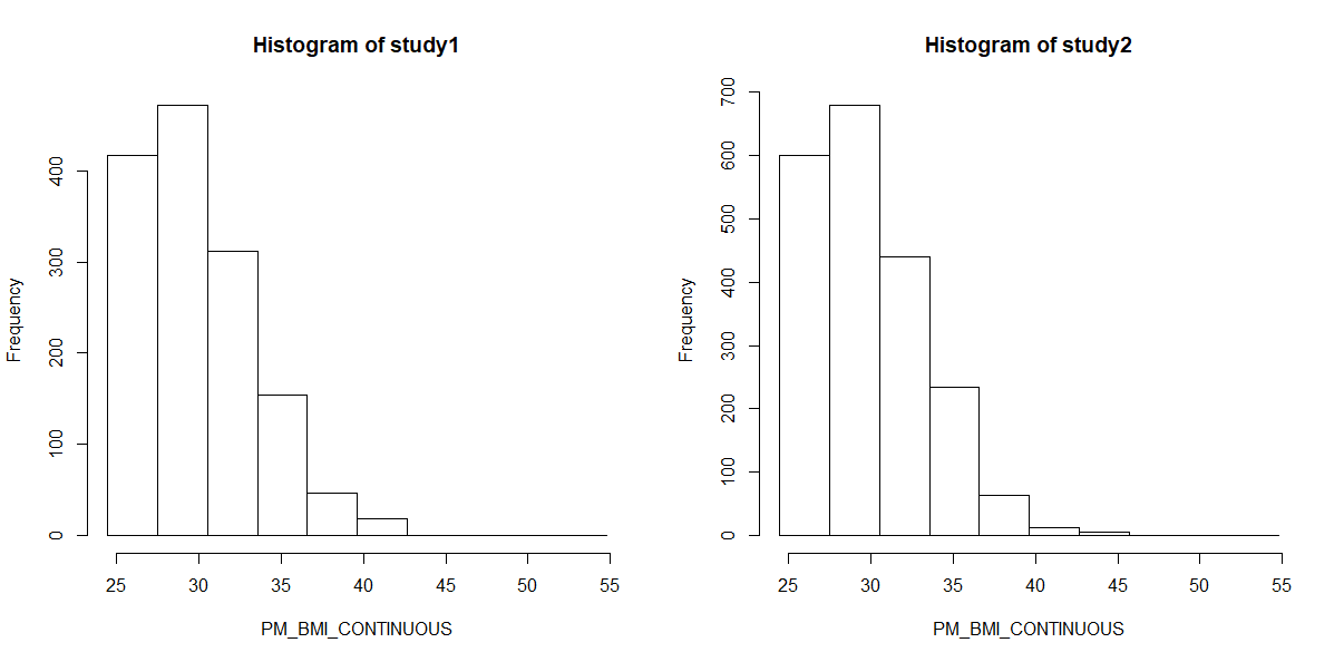
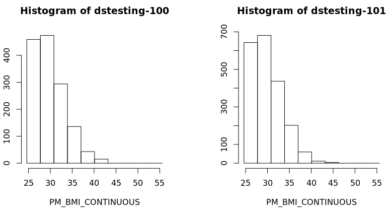
Finally we can create a histogram of these results to confirm them visually:

ds.histogram(x="subset.BMI.25.plus$PM_BMI_CONTINUOUS", datasources = connections)

Gives code output:

Aggregated (exists("subset.BMI.25.plus")) [============================================] 100% / 0s
Aggregated (classDS("subset.BMI.25.plus$PM_BMI_CONTINUOUS")) [=========================] 100% / 0s
Aggregated (histogramDS1(subset.BMI.25.plus$PM_BMI_CONTINUOUS,1,3,0.25)) [=============] 100% / 0s
Aggregated (histogramDS2(subset.BMI.25.plus$PM_BMI_CONTINUOUS,10,24.4517227951437,54.8007820545...
Warning: study1: 3 invalid cells
Warning: study2: 1 invalid cells
[[1]]
$breaks
[1] 24.45172 27.48663 30.52153 33.55644 36.59135 39.62625 42.66116 45.69606 48.73097 51.76588 54.80078

$counts
[1] 417 472 312 154 47 18 0 0 0 0

$density
[1] 0.096421960 0.109139485 0.072143049 0.035609069 0.010867703 0.004162099 0.000000000 0.000000000 0.000000000
[10] 0.000000000

$mids
[1] 25.96918 29.00408 32.03899 35.07389 38.10880 41.14371 44.17861 47.21352 50.24842 53.28333

$xname
[1] "xvect"

$equidist
[1] TRUE

attr(,"class")
[1] "histogram"

[[2]]
$breaks
[1] 24.45172 27.48663 30.52153 33.55644 36.59135 39.62625 42.66116 45.69606 48.73097 51.76588 54.80078

$counts
[1] 600 680 441 235 64 12 6 0 0 0

$density
[1] 0.0969591481 0.1098870345 0.0712649738 0.0379756663 0.0103423091 0.0019391830 0.0009695915 0.0000000000 0.0000000000
[10] 0.0000000000

$mids
[1] 25.96918 29.00408 32.03899 35.07389 38.10880 41.14371 44.17861 47.21352 50.24842 53.28333

$xname
[1] "xvect"

$equidist
[1] TRUE

attr(,"class")
[1] "histogram"

And graph:

Deprecated instructions on ds.subset and ds.subsetByClass, soon to be replaced with instructions using ds.dataFrameSubset

In DataSHIELD there are currently 3 functions that allow us to generate subset data:

ds.subsetByClass (WARNING: this function will be deprecated in the release of 6.1, all functionality has been added to ds.dataFrameSubset which will become the one-stop replacement)
ds.subset (WARNING: this function will be deprecated in the release of 6.1, all functionality has been added to ds.dataFrameSubset which will become the one-stop replacement).
ds.dataFrameSubset

Sub-setting using ds.subsetByClass

The ds.subsetByClass function generates subsets for each level of a categorical variable. If the input is a data frame it produces a subset of that data frame for each class of each categorical variable held in the data frame.
Best practice is to state the categorical variable(s) to subset using the variables argument, and the name of the subset data using the subsets argument.
The example subsets GENDER from our assigned data frame D, the subset data is named GenderTables:

ds.subsetByClass(x = 'D', subsets = "GenderTables", variables = 'GENDER', datasources = connections)

The output of ds.subsetByClass is held in a list object stored server-side, as the subset data contain individual-level records. If no name is specified in the subsets argument, the default name "subClasses" is used.

Running ds.subsetByClass on a data frame without specifying the categorical variable in the argument variableswill create a subset of all categorical variables. If the data frame holds many categorical variables the number of subsets produces might be too large - many of which may not be of interest for the analysis.

In the previous example, the GENDER variable in assigned data frame D had females coded as 0 and males coded as 1. When GENDER was subset using the ds.subsetByClass function, two subset tables were generated for each study dataset; one for females and one for males.

The ds.names function obtains the names of these subset data:

ds.names('GenderTables', datasources = connections)

  Aggregated (exists("GenderTables")) [==================================================] 100% / 0s
  Aggregated (classDS("GenderTables")) [=================================================] 100% / 0s
  Aggregated (namesDS(GenderTables)) [===================================================] 100% / 0s
$study1
[1] "GENDER.level_0" "GENDER.level_1"

$study2
[1] "GENDER.level_0" "GENDER.level_1"

Sub-setting using ds.subset

This function is soon to be deprecated. Its replacement will be ds.dataFrameSubset().

ds.dataFrameSubset() uses very different arguments to ds.subset()

Changes will be coming soon to this page. Use function help to investigate how ds.dataFrameSubset() works similarly.

The function ds.subset allows general sub-setting of different data types e.g. categorical, numeric, character, data frame, matrix. It is also possible to subset rows (the individual records). No output is returned to the client screen, the generated subsets are stored in the server-side R session.

The example below uses the function ds.subset to subset the assigned data frame D by rows (individual records) that have no missing values (missing values are denoted with NA) given by the argument completeCases=TRUE. The output subset is named "D_without_NA":

ds.subset(x='D', subset='D_without_NA', completeCases=TRUE, datasources = connections)

The ds.subset function prints an invalid message to the client screen to inform if missing values exist in a subset.

#In order to indicate that a generated subset dataframe or vector is invalid all values within it are set to NA!

An invalid message also denotes subsets that contain less than the minimum cell count determined by data providers.

The second example creates a subset of the assigned data frame D with BMI values ≥ 25 using the argument logicalOperator. The subset object is named BMI25plus using the subset argument and is not printed to client screen but is stored in the server-side R session:

ds.subset(x='D', subset='BMI25plus', logicalOperator='PM_BMI_CONTINUOUS>=', threshold=25, datasources = opals)

The subset of data retains the same variables names i.e. column names

To verify the subset above is correct (holds only observations with BMI ≥ 25) the function ds.quantileMean with the argument type='split' will confirm the BMI results for each study are ≥ 25.

ds.quantileMean('BMI25plus$PM_BMI_CONTINUOUS', type='split', datasources = opals)

$`dstesting-100`
     5%     10%     25%     50%     75%     90%     95%    Mean 
25.3500 25.7100 27.1500 29.2000 32.0600 34.6560 36.4980 29.9019 

$`dstesting-101`
      5%      10%      25%      50%      75%      90%      95%     Mean 
25.46900 25.91800 27.19000 29.27000 32.20500 34.76200 36.24300 29.92606

Also a histogram of the variable BMI of the new subset data frame could be created for each study separately:

ds.histogram('BMI25plus$PM_BMI_CONTINUOUS', datasources = opals)

ds.histogram('BMI25plus$PM_BMI_CONTINUOUS', datasources = opals)

Warning: dstesting-100: 2 invalid cells
Warning: dstesting-101: 1 invalid cells
[[1]]
$breaks
 [1] 23.93659 27.17016 30.40373 33.63731 36.87088 40.10445 43.33803 46.57160 49.80518 53.03875 56.27232
$counts
 [1] 365 511 331 150  49  15   0   0   0   0
$density
 [1] 0.079212771 0.110897880 0.071834047 0.032553194 0.010634043 0.003255319 0.000000000 0.000000000 0.000000000 0.000000000
$mids
 [1] 25.55337 28.78695 32.02052 35.25409 38.48767 41.72124 44.95482 48.18839 51.42196 54.65554
$xname
[1] "xvect"
$equidist
[1] TRUE
attr(,"class")
[1] "histogram"

[[2]]
$breaks
 [1] 23.93659 27.17016 30.40373 33.63731 36.87088 40.10445 43.33803 46.57160 49.80518 53.03875 56.27232
$counts
 [1] 506 750 476 229  62  11   4   0   0   0
$density
 [1] 0.0767450721 0.1137525773 0.0721949690 0.0347324536 0.0094035464 0.0016683711 0.0006066804 0.0000000000 0.0000000000 0.0000000000
$mids
 [1] 25.55337 28.78695 32.02052 35.25409 38.48767 41.72124 44.95482 48.18839 51.42196 54.65554
$xname
[1] "xvect"
$equidist
[1] TRUE
attr(,"class")
[1] "histogram

Conclusion