v5 Tutorial for DataSHIELD users
- Hasan Alradhi (Unlicensed)
- Alex Westerberg (Unlicensed)
- Patricia Ryser-Welch (Unlicensed)
Quick link to page for presentations etc. : http://bit.ly/intro-DS
- Introduction to DataSHIELD Extended Practical - http://bit.ly/extended-DS
- DataSHIELD extended practical answers - http://bit.ly/extended-DS-answers
- Local DataSHIELD Training Environment v5
- Function help from the manual v5
- Saving analyses to file v5
- Saving analyses to file v6
Prerequisites
It is recommended that you familiarise yourself with R first by sitting our Introduction to R tutorial.
DataSHIELD support
Free DataSHIELD support is given in the DataSHIELD forum by the DataSHIELD community.
DataSHIELD bespoke user support and also user training classes are offered on a fee basis. Please enquire at datashield@newcastle.ac.uk for current prices.
Introduction
This tutorial introduces users to DataSHIELD commands and syntax. Throughout this document we refer to R, but all commands are run in the same way in Rstudio. This tutorial contains a limited number of examples; further examples are available in each DataSHIELD function manual page that can be accessed via the help function.
The DataSHIELD approach: aggregate and assign functions
DataSHIELD commands call functions that range from carrying out pre-requisite tasks such as login to the datasources, to generating basic descriptive statistics, plots and tabulations. More advance functions allow for users to fit generalized linear models and generalized estimating equations models. R can list all functions available in DataSHIELD.
This section explains the functions we will call during this tutorial. Although this knowledge is not required to run DataSHIELD analyses it helps to understand the output of the commands. It can explain why some commands call functions that return nothing to the user, but rather store the output on the server of the data provider for use in a second function.
In DataSHIELD the person running an analysis (the client) uses client-side functions to issue commands (instructions). These commands initiate the execution (running) of server-side functions that run the analysis server-side (behind the firewall of the data provider). There are two types of server-side function: assign functions and aggregate functions.
How assign and aggregate functions work
Assign functions do not return an output to the client, with the exception of error or status messages. Assign functions create new objects and store them server-side either because the objects are potentially disclosive, or because they consist of the individual-level data which, in DataSHIELD, is never seen by the analyst. These new objects can include:
- new transformed variables (e.g. mean centred or log transformed variables)
- a new variable of a modified class (e.g. a variable of class numeric may be converted into a factor which R can then model as having discrete categorical levels)
- a subset object (e.g. a dataframe including gender as a variable may be split into males and females).
Assign functions return no output to the client except to indicate an error or useful messages about the object store on server-side.
Aggregate functions analyse the data server-side and return an output in the form of aggregate data (summary statistics that are not disclosive) to the client. The help page for each function tells us what is returned and when not to expect an output on client-side.
Starting and Logging onto the Opal Training Servers - Cloud Training Environment
If you are attending one of our training sessions you will be using our DataSHIELD Cloud Training Environment. If you are running this tutorial on a DataSHIELD VM installed on your own machine, please skip to these instructions.
Start the Opal Servers and Login
- Your trainer will have started your Opal training servers in the cloud for you.
- Your trainer will give you the IP address of the DataSHIELD client portal (RStudio) ending :8787
- They will also provide you with a username and password to login with.
DataSHIELD VMs on Local Machines
If you are using running this tutorial using the DataSHIELD VMs installed on your own machine please follow instructions to Start the Opal VMs and then continue as below.
Build your login dataframe
DataSHIELD cloud IP addresses
The DataSHIELD cloud training environment does not use fixed IP addresses, the client and opal training server addresses change each training session. As part of the user tutorial you learn how to build a DataSHIELD login dataframe. In a real world instance of DataSHIELD this is populated with secure certificates not text based usernames and passwords.
- In your DataSHIELD client R studio home directory you will have a login script similar to the template below. Double click to open it up in the top left window.
- Highlight the the login script and run it by pressing Ctrl + Enter
server <- c("dstesting-100", "dstesting-101") #The server names
url <- c("http://XXX.XXX.XXX.XXX:8080", "http://XXX.XXX.XXX.XXX:8080") #These IP addresses change
user <- "administrator"
password <- "datashield_test&"
table <- c("CNSIM.CNSIM1","CNSIM.CNSIM2") #The data tables used in the tutorial
my_logindata <- data.frame(server, url, user, password, table)
- check the login dataframe
my_logindata
Start R/RStudio and load packages
- The following relevant R packages are required for analysis
opal to login and logout
dsBaseClient containing all DataSHIELD functions referred to in this tutorial.
- To load the R packages, type the
libraryfunction into the command line as given in the example below:
#load libraries

library(opal)
Loading required package: RCurl
Loading required package: bitops
Loading required package: rjson
Loading required package: mime
library(dsBaseClient)
Log onto the remote Opal training servers
- Create a variable called
opalsthat calls thedatashield.loginfunction to log into the desired Opal servers. In the DataSHIELD test environmentmy_logindatais our login dataframe for the Opal training servers.
opals <- datashield.login(logins=my_logindata, assign=TRUE)
The output below indicates that each of the two Opal training servers
dstesting-101anddstesting-100contain the same 11 variables listed in capital letters underVariables assigned:
opals <- datashield.login(logins=my_logindata,assign=TRUE)
Logging into the collaborating servers

  No variables have been specified.
  All the variables in the opal table
  (the whole dataset) will be assigned to R!

Assigning data:
dstesting-100...
dstesting-101...

Variables assigned:
dstesting-100--LAB_TSC, LAB_TRIG, LAB_HDL, LAB_GLUC_ADJUSTED, PM_BMI_CONTINUOUS, DIS_CVA, MEDI_LPD, DIS_DIAB, DIS_AMI, GENDER, PM_BMI_CATEGORICAL
dstesting-101--LAB_TSC, LAB_TRIG, LAB_HDL, LAB_GLUC_ADJUSTED, PM_BMI_CONTINUOUS, DIS_CVA, MEDI_LPD, DIS_DIAB, DIS_AMI, GENDER, PM_BMI_CATEGORICAL
In Horizontal DataSHIELD pooled analysis, the data are harmonized and the variables given the same names across the studies, as agreed by all data providers.
How datashield.login works
The datashield.login function from the R package opal allows users to login and assign data to analyse from the Opal server in a server-side R session created behind the firewall of the data provider.
All the commands sent after login are processed within the server-side R instance only allows a specific set of commands to run (see the details of a typical horizontal DataSHIELD process). The server-side R session is wiped after logging out.
If we do not specify individual variables to assign to the server-side R session, all variables held in the Opal servers are assigned. Assigned data are kept in a data frame named D by default. Each column of that data frame represents one variable and the rows are the individual records.
Assign individual variables on login
Users can specify individual variables to assign to the server-side R session. It is best practice to first create a list of the Opal variables you want to analyse.
- The example below creates a new variable
myvarthat lists the Opal variables required for analysis:LAB_HDLandGENDER - The
variablesargument in the functiondatashield.loginusesmyvar, which then will call only this list.
myvar <- list('LAB_HDL', 'GENDER')
opals <- datashield.login(logins=my_logindata, assign=TRUE, variables=myvar)

Logging into the collaborating servers

Assigning data:
dstesting-100...
dstesting-101...

Variables assigned:
dstesting-100--LAB_HDL, GENDER
dstesting-101--LAB_HDL, GENDER
The format of assigned data frames
Assigned data are kept in a data frame (table) named D by default. Each row of the data frame are the individual records and each column is a separate variable.
- The example below uses the argument
symbolin thedatashield.loginfunction to change the name of the data frame fromDtomytable
myvar <- list('LAB_HDL', 'GENDER')
opals <- datashield.login(logins=my_logindata, assign=TRUE, variables=myvar, symbol='mytable')

Logging into the collaborating servers

Assigning data:
dstesting-100...
dstesting-101...

Variables assigned:
dstesting-100--LAB_HDL, GENDER
dstesting-101--LAB_HDL, GENDER
Only DataSHIELD developers will need to change the default value of the last argument, directory, of the datashield.login function.
Basic statistics and data manipulations
Descriptive statistics: variable dimensions and class
Almost all functions in DataSHIELD can display split results (results separated for each study) or pooled results (results for all the studies combined). This can be done using the type='split' and type='combine' argument in each function. The majority of DataSHIELD functions have a default of type='combine'. The default for each function can be checked in the function help page. Some of the new versions of functions include the option type='both' which returns both the split and the pooled results.
It is possible to get some descriptive or exploratory statistics about the assigned variables held in the server-side R session such as number of participants at each data provider, number of participants across all data providers and number of variables. Identifying parameters of the data will facilitate your analysis.
- The dimensions of the assigned data frame
Dcan be found using theds.dimcommand in whichtype='both'is the default argument:
opals <- datashield.login(logins=my_logindata, assign=TRUE)
ds.dim(x = 'D')
The output of the command is shown below. It shows that in study 1 (dstesting-100) there are 2163 individuals with 11 variables and in study 2 (dstesting-101) there are 3088 individuals with 11 variables, and that in both studies together there are in total 5251 individuals with 11 variables:
$`dimensions of D in dstesting-100`
[1] 2163   11

$`dimensions of D in dstesting-101`
[1] 3088   11

$`dimensions of D in combined studies`
[1] 5251   11
- Use the
type='combine'argument in theds.dimfunction to identify the number of individuals (5251) and variables (11) pooled across all studies:
ds.dim(x='D', type='combine', datasources = opals)
$`dimensions of D in combined studies`
[1] 5251   11
- To check the variables in each study are identical (as is required for pooled data analysis), use the
ds.colnamesfunction on the assigned data frameD:
ds.colnames(x='D', datasources = opals)

$`dstesting-100`
 [1] "LAB_TSC"            "LAB_TRIG"           "LAB_HDL"            "LAB_GLUC_ADJUSTED"  "PM_BMI_CONTINUOUS"  "DIS_CVA"            "MEDI_LPD"
 [8] "DIS_DIAB"           "DIS_AMI"            "GENDER"             "PM_BMI_CATEGORICAL"

$`dstesting-101`
 [1] "LAB_TSC"            "LAB_TRIG"           "LAB_HDL"            "LAB_GLUC_ADJUSTED"  "PM_BMI_CONTINUOUS"  "DIS_CVA"            "MEDI_LPD"
 [8] "DIS_DIAB"           "DIS_AMI"            "GENDER"             "PM_BMI_CATEGORICAL"
- Use the
ds.classfunction to identify the class (type) of a variable - for example if it is an integer, character, factor etc. This will determine what analysis you can run using this variable class. The example below defines the class of the variableLAB_HDLheld in the assigned data frameD, denoted by the argumentx='D$LAB_HDL'.
ds.class(x='D$LAB_HDL', datasources = opals)

$`dstesting-100`
[1] "numeric"

$`dstesting-101`
[1] "numeric"
Descriptive statistics: quantiles and mean
As LAB_HDL is a numeric variable the distribution of the data can be explored.
- The function
ds.quantileMeanreturns the quantiles and the statistical mean. It does not return minimum and maximum values as these values are potentially disclosive (e.g. the presence of an outlier). By defaulttype='combined'in this function - the results reflect the quantiles and mean pooled for all studies. Specifying the argumenttype='split'will give the quantiles and mean for each study:
ds.quantileMean(x='D$LAB_HDL', datasources = opals)

Quantiles of the pooled data
       5%       10%       25%       50%       75%       90%       95%
0.8606589 1.0385205 1.2964949 1.5704848 1.8418712 2.0824057 2.2191369

Mean
1.5619572
- To get the statistical mean alone, use the function
ds.meanuse the argumenttypeto request split results:
ds.mean(x='D$LAB_HDL', datasources = opals)

$Mean.by.Study
              EstimatedMean Nmissing Nvalid Ntotal
dstesting-100      1.569416      360   1803   2163
dstesting-101      1.556648      555   2533   3088

$Nstudies
[1] 2

$ValidityMessage
              ValidityMessage
dstesting-100 "VALID ANALYSIS"
dstesting-101 "VALID ANALYSIS"
Descriptive statistics: assigning variables
So far all the functions in this section have returned something to the screen. Some functions (assign functions) create new objects in the server-side R session that are required for analysis but do not return an anything to the client screen. For example, in analysis the log values of a variable may be required.
- By default the function
ds.logcomputes the natural logarithm. It is possible to compute a different logarithm by setting the argumentbaseto a different value. There is no output to screen:
ds.log(x='D$LAB_HDL', datasources = opals)
- In the above example the name of the new object was not specified. By default the name of the new variable is set to the input vector followed by the suffix '_log' (i.e. '
LAB_HDL_log')
- It is possible to customise the name of the new object by using the
newobjargument:
ds.log(x='D$LAB_HDL', newobj='LAB_HDL_log', datasources = opals)
- The new object is not attached to assigned variables data frame (default name
D). We can check the size of the new LAB_HDL_log vector we generated above; the command should return the same figure as the number of rows in the data frame 'D'.
ds.length(x='LAB_HDL_log', datasources = opals)

$`length of LAB_HDL_log in dstesting-100`
[1] 2163

$`length of LAB_HDL_log in dstesting-101`
[1] 3088

$`total length of LAB_HDL_log in all studies combined`
[1] 5251
ds.assign
The ds.assign function enables the creation of new objects in the server-side R session to be used in later analysis. ds.assign can be used to evaluate simple expressions passed on to its argument toAssign and assign the output of the evaluation to a new object.
- Using
ds.assignwe subtract the pooled mean calculated earlier from LAB_HDL (mean centring) and assign the output to a new variable calledLAB_HDL.c. The function returns no output to the client screen, the newly created variable is stored server-side.
ds.assign(toAssign='D$LAB_HDL-1.562', newobj='LAB_HDL.c', datasources = opals)
Further DataSHIELD functions can now be run on this new mean-centred variable
LAB_HDL.c. The example below calculates the mean of the new variable
LAB_HDL.c
which should be approximately 0.
ds.mean(x='LAB_HDL.c', datasources = opals)

$Mean.by.Study
              EstimatedMean Nmissing Nvalid Ntotal
dstesting-100   0.007416316      360   1803   2163
dstesting-101  -0.005352231      555   2533   3088

$Nstudies
[1] 2

$ValidityMessage
              ValidityMessage
dstesting-100 "VALID ANALYSIS"
dstesting-101 "VALID ANALYSIS"
Generating contingency tables
The function
ds.table1D
creates a one-dimensional contingency table of a categorical variable. The default is set to run on pooled data from all studies, to obtain an output of each study set the argument
type='split'
.
- The example below calculates a one-dimensional table for the variable
GENDER. The function returns the counts and the column and row percent per category, as well as information about the validity of the variable in each study dataset:
ds.table1D(x='D$GENDER')

$counts
      D$GENDER
0         2677
1         2574
Total     5251

$percentages
      D$GENDER
0        50.98
1        49.02
Total   100.00

$validity
[1] "All tables are valid!"
In DataSHIELD tabulated data are flagged as invalid if one or more cells have a count of between 1 and the minimal cell count allowed by the data providers. For example data providers may only allow cell counts ≥ 5).
The function
ds.table2D
creates two-dimensional contingency tables of a categorical variable. Similar to
ds.table1D
the default is set to run on pooled data from all studies, to obtain an output of each study set the argument type='split'.
- The example below constructs a two-dimensional table comprising cross-tabulation of the variables
DIS_DIAB(diabetes status) andGENDER. The function returns the same output asds.table1Dbut additionally computes a chi-squared test for homogeneity on (nc-1)*(nr-1) degrees of freedom (where nc is the number of columns and nr is the number of rows):
ds.table2D(x='D$DIS_DIAB', y='D$GENDER', datasources = opals)

$colPercent
$colPercent$`dstesting-100-D$DIS_DIAB(row)|D$GENDER(col)`
           0      1  Total
0      98.08  99.16  98.61
1       1.92   0.84   1.39
Total 100.00 100.00 100.00

$colPercent$`dstesting-101-D$DIS_DIAB(row)|D$GENDER(col)`
           0      1  Total
0      98.04  98.94  98.48
1       1.96   1.06   1.52
Total 100.00 100.00 100.00
$colPercent.all.studies
$colPercent.all.studies$`pooled-D$DIS_DIAB(row)|D$GENDER(col)`
           0      1  Total
0      98.06  99.03  98.53
1       1.94   0.97   1.47
Total 100.00 100.00 100.00

$rowPercent
$rowPercent$`dstesting-100-D$DIS_DIAB(row)|D$GENDER(col)`
          0     1 Total
0     50.21 49.79   100
1     70.00 30.00   100
Total 50.49 49.51   100

$rowPercent$`dstesting-101-D$DIS_DIAB(row)|D$GENDER(col)`
          0     1 Total
0     51.10 48.90   100
1     65.96 34.04   100
Total 51.33 48.67   100

$rowPercent.all.studies
$rowPercent.all.studies$`pooled-D$DIS_DIAB(row)|D$GENDER(col)`
          0     1 Total
0     50.73 49.27   100
1     67.53 32.47   100
Total 50.98 49.02   100

$chi2Test
$chi2Test$`dstesting-100-D$DIS_DIAB(row)|D$GENDER(col)`

	Pearson's Chi-squared test with Yates' continuity correction

data:  contingencyTable
X-squared = 3.8767, df = 1, p-value = 0.04896

$chi2Test$`dstesting-101-D$DIS_DIAB(row)|D$GENDER(col)`

	Pearson's Chi-squared test with Yates' continuity correction

data:  contingencyTable
X-squared = 3.5158, df = 1, p-value = 0.06079
$chi2Test.all.studies
$chi2Test.all.studies$`pooled-D$DIS_DIAB(row)|D$GENDER(col)`

	Pearson's Chi-squared test with Yates' continuity correction

data:  pooledContingencyTable
X-squared = 7.9078, df = 1, p-value = 0.004922

$counts
$counts$`dstesting-100-D$DIS_DIAB(row)|D$GENDER(col)`
         0    1 Total
0     1071 1062  2133
1       21    9    30
Total 1092 1071  2163

$counts$`dstesting-101-D$DIS_DIAB(row)|D$GENDER(col)`
         0    1 Total
0     1554 1487  3041
1       31   16    47
Total 1585 1503  3088

$counts.all.studies
$counts.all.studies$`pooled-D$DIS_DIAB(row)|D$GENDER(col)`
         0    1 Total
0     2625 2549  5174
1       52   25    77
Total 2677 2574  5251

$validity
[1] "All tables are valid!"
Generating graphs
It is currently possible to produce 4 types of graphs in DataSHIELD: histograms, contour plots, heatmap plots, scatter plots
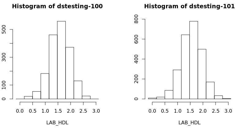
Histograms
Histograms
In the default method of generating a DataSHIELD histogram outliers are not shown as these are potentially disclosive. The text summary of the function printed to the client screen informs the user of the presence of classes (bins) with a count smaller than the minimal cell count set by data providers.
- The
ds.histogramfunction can be used to create a histogram ofLAB_HDLthat is in the assigned variable dataframe (named D, by default). The default analysis is set to run on separate data from all studies. Note that dstesting-100 contain 2 invalid cells (bins) - those bins contain counts less than the data provider minimal cell count. - Note that a small random number is added to the minimum and maximum values of the range of the input variable. Therefore each user should expect slightly different printed results from those shown below:
ds.histogram(x='D$LAB_HDL', datasources = opals)

Warning: dstesting-100: 2 invalid cells
Warning: dstesting-101: 0 invalid cells
[[1]]
$breaks
 [1] -0.1489566  0.1799465  0.5088497  0.8377529  1.1666561  1.4955593  1.8244625  2.1533657  2.4822688  2.8111720  3.1400752
$counts
 [1]   0  21  55 200 468 573 353 111  20   0
$density
 [1] 0.00000000 0.03541241 0.09274679 0.33726105 0.78919086 0.96625291 0.59526576 0.18717988 0.03372611 0.00000000
$mids
 [1] 0.01549495 0.34439814 0.67330132 1.00220451 1.33110769 1.66001088 1.98891406 2.31781725 2.64672043 2.97562362
$xname
[1] "xvect"
$equidist
[1] TRUE
attr(,"class")
[1] "histogram"

[[2]]
$breaks
 [1] -0.1489566  0.1799465  0.5088497  0.8377529  1.1666561  1.4955593  1.8244625  2.1533657  2.4822688  2.8111720  3.1400752
$counts
 [1]   9  21  88 308 678 768 472 155  30   4
$density
 [1] 0.010802872 0.025206702 0.105628084 0.369698295 0.813816376 0.921845098 0.566550633 0.186049466 0.036009574 0.004801277
$mids
 [1] 0.01549495 0.34439814 0.67330132 1.00220451 1.33110769 1.66001088 1.98891406 2.31781725 2.64672043 2.97562362
$xname
[1] "xvect"
$equidist
[1] TRUE
attr(,"class")
[1] "histogram"
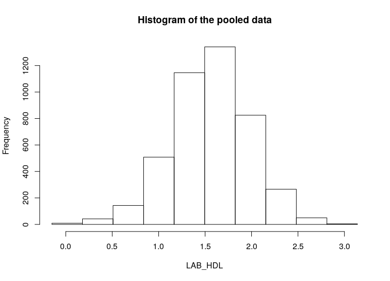
- To produce histograms from a pooled study, the argument
type='combine'is used.
ds.histogram(x='D$LAB_HDL', type = 'combine', datasources = opals)

$breaks
 [1] -0.1489566  0.1799465  0.5088497  0.8377529  1.1666561  1.4955593  1.8244625  2.1533657  2.4822688  2.8111720  3.1400752

$counts
 [1]    9   42  143  508 1146 1341  825  266   50    4

$density
 [1] 0.003600957 0.020206371 0.066124958 0.235653115 0.534335745 0.629366003 0.387272130 0.124409783 0.023245226 0.001600426

$mids
 [1] 0.01549495 0.34439814 0.67330132 1.00220451 1.33110769 1.66001088 1.98891406 2.31781725 2.64672043 2.97562362

$xname
[1] "xvect"

$equidist
[1] TRUE

$intensities
 [1] 0.003600957 0.020206371 0.066124958 0.235653115 0.534335745 0.629366003 0.387272130 0.124409783 0.023245226 0.001600426

attr(,"class")
[1] "histogram
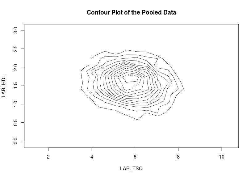
Contour plots
Contour plots are used to visualize a correlation pattern.
- The function
ds.contourPlotis used to visualise the correlation between the variablesLAB_TSC(total serum cholesterol andLAB_HDL(HDL cholesterol). The default istype='combined'- the results represent a contour plot on pooled data across all studies:
ds.contourPlot(x='D$LAB_TSC', y='D$LAB_HDL', datasources = opals)

dstesting-100: Number of invalid cells (cells with counts >0 and < nfilter.tab ) is 53
dstesting-101: Number of invalid cells (cells with counts >0 and < nfilter.tab ) is 72
Heat map plots
An alternative way to visualise correlation between variables is via a heat map plot.
- The function
ds.heatmapPlotis applied to the variablesLAB_TSCandLAB_HDL:
ds.heatmapPlot(x='D$LAB_TSC', y='D$LAB_HDL', datasources = opals)

dstesting-100: Number of invalid cells (cells with counts >0 and < nfilter.tab ) is 53
dstesting-101: Number of invalid cells (cells with counts >0 and < nfilter.tab ) is 72
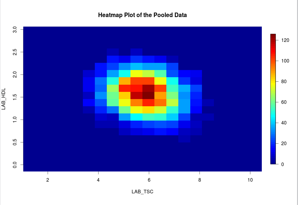
The functions ds.contourPlot and ds.heatmapPlot use the range (minimum and maximum values) of the x and y vectors in the process of generating the graph. But in DataSHIELD the minimum and maximum values cannot be returned because they are potentially disclosive; hence what is actually returned for these plots is the 'obscured' minimum and maximum.
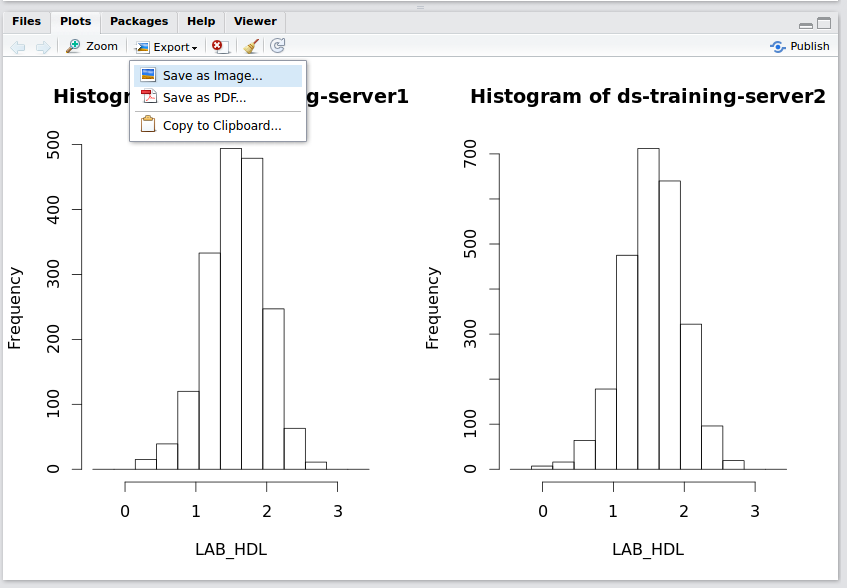
Saving Graphs / Plots in R Studio
- Any plots will appear in the bottom right window in R Studio, within the
plottab - Select
export>save as image
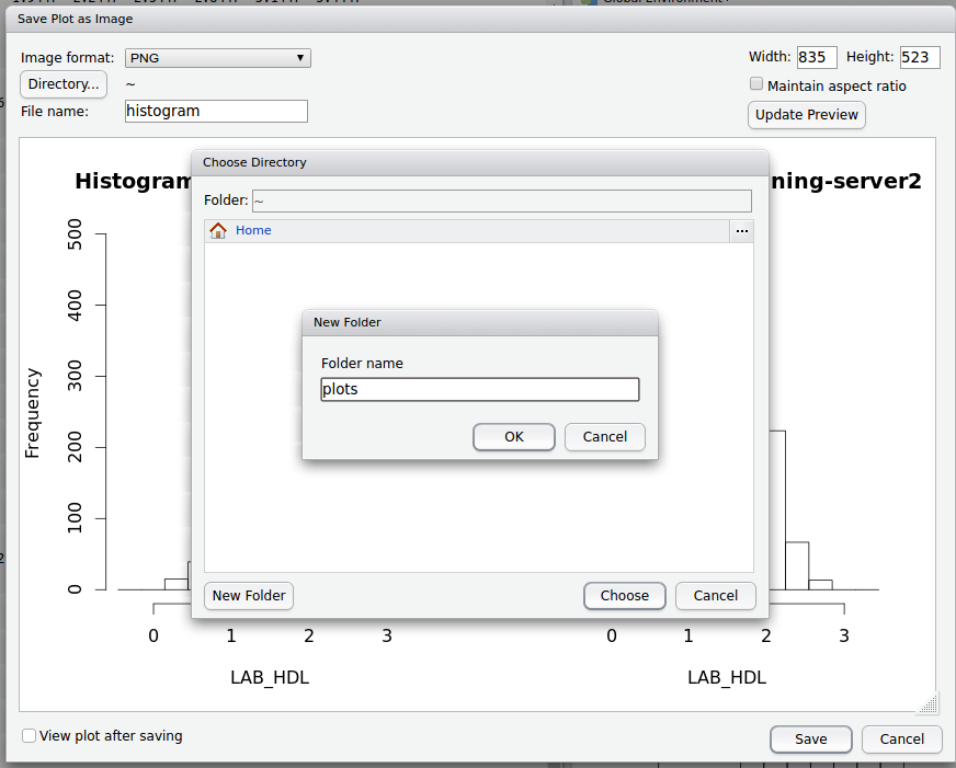
- Name the file and select / create a folder to store the image in on the DataSHIELD Client server.
- You can also edit the width and height of the graph
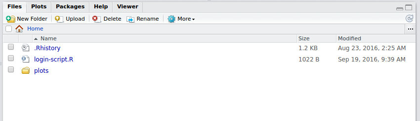
- The plot will now be accessible from your Home folder directory structure. On a live DataSHIELD system you can then transfer the plot to your computer via secure file transfer (sftp).
Sub-setting
Limitations on subsetting
Sub-setting is particularly useful in statistical analyses to break down variables or tables of variables into groups for analysis. Repeated sub-setting, however, can lead to thinning of the data to individual-level records that are disclosive (e.g. the statistical mean of a single value point is the value itself). Therefore, DataSHIELD does not subset an object below the minimal subset length set by the data providers (typically this is ≤ 4 observations).
In DataSHIELD there are currently 3 functions that allow us to generate subsets data:
- ds.subsetByClass
- ds.subset
- ds.dataFrameSubset
Sub-setting using ds.subsetByClass
- The
ds.subsetByClassfunction generates subsets for each level of acategoricalvariable. If the input is a data frame it produces a subset of that data frame for each class of each categorical variable held in the data frame. - Best practice is to state the categorical variable(s) to subset using the
variablesargument, and the name of the subset data using thesubsetsargument. - The example subsets
GENDERfrom our assigned data frameD, the subset data is namedGenderTables:
ds.subsetByClass(x = 'D', subsets = "GenderTables", variables = 'GENDER', datasources = opals)
- The output of
ds.subsetByClassis held in alistobject stored server-side, as the subset data contain individual-level records. If no name is specified in thesubsetsargument, the default name ofsubClassesis used.
Running ds.subsetByClass on a data frame without specifying the categorical variable in the argument
variables
will create a subset of all categorical variables. If the data frame holds many categorical variables the number of subsets produces might be too large - many of which may not be of interest for the analysis.
In the previous example, the
GENDER
variable in assigned data frame
D
had females coded as 0 and males coded as 1. When
GENDER
was subset using the ds.subsetByClass function, two subset tables were generated for each study dataset; one for females and one for males.
- The
ds.namesfunction obtains the names of these subset data:
ds.names('GenderTables', datasources = opals)

$`dstesting-100`
[1] "GENDER.level_0" "GENDER.level_1"

$`dstesting-101`
[1] "GENDER.level_0" "GENDER.level_1"
Sub-setting using ds.subset
The function
ds.subset
allows general sub-setting of different data types e.g. categorical, numeric, character, data frame, matrix. It is also possible to subset rows (the individual records). No output is returned to the client screen, the generated subsets are stored in the server-side R session.
- The example below uses the function
ds.subsetto subset the assigned data frameDby rows (individual records) that have no missing values (missing values are denoted withNA) given by the argumentcompleteCases=TRUE. The output subset is namedD_without_NA:
ds.subset(x='D', subset='D_without_NA', completeCases=TRUE, datasources = opals)
The ds.subset function prints an invalid message to the client screen to inform if missing values exist in a subset.
#In order to indicate that a generated subset dataframe or vector is invalid all values within it are set to NA!
An invalid message also denotes subsets that contain less than the minimum cell count determined by data providers.
- The second example creates a subset of the assigned data frame
Dwith BMI values ≥ 25 using the argumentlogicalOperator. The subset object is namedBMI25plususing thesubsetargument and is not printed to client screen but is stored in the server-side R session:
ds.subset(x='D', subset='BMI25plus', logicalOperator='PM_BMI_CONTINUOUS>=', threshold=25, datasources = opals)
The subset of data retains the same variables names i.e. column names
- To verify the subset above is correct (holds only observations with BMI ≥ 25) the function
ds.quantileMeanwith the argumenttype='split'will confirm the BMI results for each study are ≥ 25.
ds.quantileMean('BMI25plus$PM_BMI_CONTINUOUS', type='split', datasources = opals)

$`dstesting-100`
     5%     10%     25%     50%     75%     90%     95%    Mean
25.3500 25.7100 27.1500 29.2000 32.0600 34.6560 36.4980 29.9019

$`dstesting-101`
      5%      10%      25%      50%      75%      90%      95%     Mean
25.46900 25.91800 27.19000 29.27000 32.20500 34.76200 36.24300 29.92606
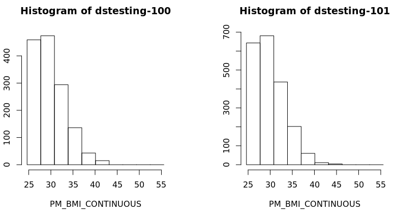
- Also a histogram of the variable BMI of the new subset data frame could be created for each study separately:
ds.histogram('BMI25plus$PM_BMI_CONTINUOUS', datasources = opals)

Warning: dstesting-100: 2 invalid cells
Warning: dstesting-101: 1 invalid cells
[[1]]
$breaks
 [1] 23.93659 27.17016 30.40373 33.63731 36.87088 40.10445 43.33803 46.57160 49.80518 53.03875 56.27232
$counts
 [1] 365 511 331 150  49  15   0   0   0   0
$density
 [1] 0.079212771 0.110897880 0.071834047 0.032553194 0.010634043 0.003255319 0.000000000 0.000000000 0.000000000 0.000000000
$mids
 [1] 25.55337 28.78695 32.02052 35.25409 38.48767 41.72124 44.95482 48.18839 51.42196 54.65554
$xname
[1] "xvect"
$equidist
[1] TRUE
attr(,"class")
[1] "histogram"

[[2]]
$breaks
 [1] 23.93659 27.17016 30.40373 33.63731 36.87088 40.10445 43.33803 46.57160 49.80518 53.03875 56.27232
$counts
 [1] 506 750 476 229  62  11   4   0   0   0
$density
 [1] 0.0767450721 0.1137525773 0.0721949690 0.0347324536 0.0094035464 0.0016683711 0.0006066804 0.0000000000 0.0000000000 0.0000000000
$mids
 [1] 25.55337 28.78695 32.02052 35.25409 38.48767 41.72124 44.95482 48.18839 51.42196 54.65554
$xname
[1] "xvect"
$equidist
[1] TRUE
attr(,"class")
[1] "histogram
Modelling
Horizontal DataSHIELD allows the fitting of generalised linear models (GLM). In the GLM function the outcome can be modelled as continuous, or categorical (binomial or discrete). The error to use in the model can follow a range of distribution including gaussian, binomial, Gamma and poisson. In this section only one example will be shown, for more examples please see the manual help page for the function.
Generalised linear models
- The function
ds.glmis used to analyse the outcome variableDIS_DIAB(diabetes status) and the covariatesPM_BMI_CONTINUOUS(continuous BMI),LAB_HDL(HDL cholesterol) andGENDER(gender), with an interaction between the latter two. In R this model is represented as:
D$DIS_DIAB ~ D$PM_BMI_CONTINUOUS+D$LAB_HDL*D$GENDER
- By default intermediate results are not printed to the client screen. It is possible to display the intermediate results, to show the coefficients after each iteration, by using the argument
display=TRUE.
ds.glm(formula=D$DIS_DIAB~D$PM_BMI_CONTINUOUS+D$LAB_HDL*D$GENDER, family='binomial')

Iteration 1...
CURRENT DEVIANCE:      2401.06183345965
Iteration 2...
CURRENT DEVIANCE:      555.494312555984
Iteration 3...
CURRENT DEVIANCE:      313.944280815433
Iteration 4...
CURRENT DEVIANCE:      254.951394050969
Iteration 5...
CURRENT DEVIANCE:      243.362297465085
Iteration 6...
CURRENT DEVIANCE:      242.159478947391
Iteration 7...
CURRENT DEVIANCE:      242.136131635842
Iteration 8...
CURRENT DEVIANCE:      242.136118930087
Iteration 9...
CURRENT DEVIANCE:      242.136118930082
SUMMARY OF MODEL STATE after iteration 9
Current deviance 242.136118930082 on 1727 degrees of freedom
Convergence criterion TRUE (2.02981939818773e-14)

beta: -6.01092103665866 0.105775545626623 -0.779525500352656 -0.608364943883935 0.201270260609118

Information matrix overall:
                     (Intercept)  D$M_BMI_CONTINUOUS D$LAB_HDL
(Intercept)          23.471800    706.2480           33.18849
D$M_BMI_CONTINUOUS   706.247983   21826.3834         992.20214
D$LAB_HDL            33.188486    992.2021           51.47329
D$GENDER1            8.871414     260.4081           13.51434
D$LAB_HDL:D$GENDER1  13.514336    395.4327           21.98133

                    D$GENDER1     D$LAB_HDL:D$GENDER1
(Intercept)         8.871414      13.51434
D$M_BMI_CONTINUOUS  260.40808     395.43267
D$LAB_HDL           13.514336     21.98133
D$GENDER1           8.871414      13.51434
D$LAB_HDL:D$GENDER1 13.514336     21.98133
Score vector overall:
                             [,1]
(Intercept)         -2.236579e-12
D$PM_BMI_CONTINUOUS -6.009415e-11
D$LAB_HDL           -4.135553e-12
D$GENDER1           -2.105691e-12
D$LAB_HDL:D$GENDER1 -3.929211e-12
Current deviance: 242.136118930082

$Nvalid
[1] 1732

$Nmissing
[1] 431

$Ntotal
[1] 2163

$disclosure.risk
              RISK OF DISCLOSURE
dstesting-100                  0
dstesting-101                  0

$errorMessage
              ERROR MESSAGES
dstesting-100 "No errors"
dstesting-101 "No errors"

$nsubs
[1] 1732

$iter
[1] 9

$family
Family: binomial
Link function: logit
$formula
[1] "D$DIS_DIAB ~ D$PM_BMI_CONTINUOUS + D$LAB_HDL * D$GENDER"

$coefficients
                    Estimate       Std. Error  z-value     p-value
(Intercept)         -6.0109210     1.59383740  -3.7713515  0.0001623658
D$PM_BMI_CONTINUOUS  0.1057755     0.04219371   2.5069032  0.0121794058
D$LAB_HDL           -0.7795255     0.58196551  -1.3394703  0.1804176284
D$GENDER1           -0.6083649     1.56828457  -0.3879174  0.6980771283
D$LAB_HDL:D$GENDER1  0.2012703     1.02620174   0.1961313  0.8445074133

                    low0.95CI.LP   high0.95CI.LP  P_OR
(Intercept)         -9.13478494    -2.8870571     0.002445832
D$PM_BMI_CONTINUOUS  0.02307739    0.1884737     1.111572351
D$LAB_HDL           -1.92015695    0.3611059     0.458623576
D$GENDER1           -3.68214623    2.4654163     0.544240005
D$LAB_HDL:D$GENDER1 -1.81004818    2.2125887     1.222955244

                    low0.95CI.P_OR high0.95CI.P_OR
(Intercept)         0.0001078367   0.0527971
D$PM_BMI_CONTINUOUS 1.0233457381   1.2074053
D$LAB_HDL           0.1465839544   1.4349155
D$GENDER1           0.0251688987   11.7683808
D$LAB_HDL:D$GENDER1 0.1636462519   9.1393448

$dev
[1] 242.1361
$df
[1] 1727
$output.information
[1] "SEE TOP OF OUTPUT FOR INFORMATION ON MISSING DATA AND ERROR MESSAGES"
How ds.glm works
After every iteration in the glm, each study returns non disclosive summaries (a score vector and an information matrix) that are combined on the client R session. The model is fitted again with the updated beta coefficients, this iterative process continues until convergence or the maximum number of iterations is reached. The output of ds.glm returns the final pooled score vector and information along with some information about the convergence and the final pooled beta coefficients.
You have now sat our basic DataSHIELD training. If you would like to practice further please sit our
Also remember you can:
- get a function list for any DataSHIELD package and
- view the manual help page individual functions
- in the DataSHIELD test environment it is possible to print analyses to file (.csv, .txt, .pdf, .png)
- take a look at our FAQ page for solutions to common problems such as Changing variable class to use in a specific DataSHIELD function.
- Get support from our DataSHIELD forum.
Related content

DataSHIELD Wiki by DataSHIELD is licensed under a Creative Commons Attribution-ShareAlike 4.0 International License. Based on a work at http://www.datashield.ac.uk/wiki